HYDRODYNAMICS OF PUMPS
by Christopher Earls Brennen © Concepts NREC 1994
CHAPTER 8.
PUMP VIBRATION
8.1 INTRODUCTION
The trend toward higher speed, high power density liquid turbomachinery has inevitably increased the potential for fluid/structure interaction problems, and the severity of those problems. Even in the absence of cavitation and its complications, these fluid structure interaction phenomena can lead to increased wear and, under the worst conditions, to structural failure. Exemplifying this trend, the Electrical Power Research Institute (Makay and Szamody 1978) has recognized that the occurrence of these problems in boiler feed pumps has contributed significantly to downtime in conventional power plants.
Unlike the cavitation issues, unsteady flow problems in liquid turbomachines do not have a long history of research. In some ways this is ironic since, as pointed out by Ek (1957) and Dean (1959), the flow within a turbomachine must necessarily be unsteady if work is to be done on or by the fluid. Yet many of the classical texts on pumps or turbines barely make mention of unsteady flow phenomena or of design considerations that might avoid such problems. In contrast to liquid turbomachinery, the literature on unsteady flow problems in gas turbomachinery is considerably more extensive, and there are a number of review papers that provide a good survey of the subject (for example, McCroskey 1977, Cumpsty 1977, Mikolajczak et al. 1975, Platzer 1978, Greitzer 1981). We will not attempt a review of this literature but we will try, where appropriate, to indicate areas of useful cross-reference. It is also clear that this subject incorporates a variety of problems ranging, for example, from blade flutter to fluid-induced rotordynamic instability. Because of this variety and the recent vintage of the fundamental research, no clear classification system for these problems has yet evolved and there may indeed be some phenomena that have yet to be properly identified. It follows that the classification system that we will attempt here will be tentative, and not necessarily comprehensive. Nevertheless, it seems that three different categories of flow oscillation can occur, and that there are a number phenomena within each of the three categories. We briefly list them here and return to some in the sections that follow.
- [A] Global Flow Oscillations.
A number of the identified vibration problems involve large scale
oscillations of the flow. Specific examples are:
- [A1] Rotating stall or rotating cavitation occurs when a turbomachine is required to operate at a high incidence angle close to the value at which the blades may stall. It is often the case that stall will first be manifest on a small number of adjacent blades and that this ``stall cell'' will propagate circumferentially at some fraction of the main impeller rotation speed. This phenomenon is called rotating stall and is usually associated with turbomachines having a substantial number of blades (such as compressors). It has, however, also been reported in centrifugal pumps. When the turbomachine cavitates the same phenomenon may still occur, perhaps in some slightly altered form. Such circumstances will be referred to as ``rotating stall with cavitation.'' But there is also a different phenomenon which can occur in which one or two blades manifest a greater degree of cavitation and this ``cell'' propagates around the rotor in a manner superficially similar to the propagation of rotating stall. This phenomenon is known as ``rotating cavitation.''
- [A2] Surge is manifest in a turbomachine that is required to operate under highly loaded circumstances where the slope of the head rise/flow rate curve is positive. It is a system instability to which the dynamics of all the components of the system (reservoirs, valves, inlet and suction lines and turbomachine) contribute. It results in pressure and flow rate oscillations throughout the system. When cavitation is present the phenomenon is termed ``auto-oscillation'' and can occur even when the slope of the head rise/flow rate curve is negative.
- [A3] Partial cavitation or supercavitation can become unstable when the length of the cavity approaches the length of the blade so that the cavity collapses in the region of the trailing edge. Such a circumstance can lead to violent oscillations in which the cavity length oscillates dramatically.
- [A4] Line resonance occurs when one of the blade passing frequencies in a turbomachine happens to coincide with one of the acoustic modes of the inlet or discharge line. The pressure oscillation magnitudes associated with these resonances can often cause substantial damage.
- [A5] It has been speculated that an axial balance resonance could occur if the turbomachine is fitted with a balance piston (designed to equalize the axial forces acting on the impeller) and if the resonant frequency of the balance piston system corresponds with the rotating speed or some blade passing frequency. Though there exist several apocryphal accounts of such resonances, the phenomenon has yet to be documented experimentally.
- [A6] Cavitation noise can sometimes reach a sufficient amplitude to cause resonance with structural frequencies of vibration.
- [A7] The above items all assume that the turbomachine is fixed in a non-accelerating reference frame. When this is not the case the dynamics of the turbomachine may play a crucial role in generating an instability that involves the vibration of that machine as a whole. Such phenomena, of which the Pogo instabilities are, perhaps, the best documented examples, are described further in section 8.13.
- [B] Local Flow Oscillations.
Several other vibration problems involve more localized flow oscillations
and vibration of the blades:
- [B1] Blade flutter. As in the case of airfoils, there are circumstances under which an individual blade may begin to flutter (or diverge) as a consequence of the particular flow condition (incidence angle, velocity), the stiffness of the blade, and its method of support.
- [B2] Blade excitation due to rotor-stator interaction. While [B1] would occur in the absence of excitation it is also true that there are a number of possible mechanisms of excitation in a turbomachine that can cause significant blade vibration. This is particularly true for a row of stator blades operating just downstream of a row of impeller blades or vice versa. The wakes from the upstream blades can cause a serious vibration problem for the downstream blades at blade passing frequency or some multiple thereof. Non-axisymmetry in the inlet, the volute, or housing can also cause excitation of impeller blades at the impeller rotation frequency.
- [B3] Blade excitation due to vortex shedding or cavitation oscillations. In addition to the excitation of [B2], it is also possible that vortex shedding or the oscillations of cavitation could provide the excitation for blade vibrations.
- [C] Radial and Rotordynamic Forces.
Global forces perpendicular to the axis of rotation can generate several
types of problem:
- [C1] Radial forces are forces perpendicular to the axis of rotation caused by circumferential nonuniformities in the inlet flow, casing, or volute. While these may be stationary in the frame of the pump housing, the loads that act on the impeller and, therefore, the bearings can be sufficient to create wear, vibration, and even failure of the bearings.
- [C2] Fluid-induced rotordynamic forces occur as the result of movement of the axis of rotation of the impeller-shaft system of the turbomachine. Contributions to these rotordynamic forces can arise from the seals, the flow through the impeller, leakage flows, or the flows in the bearings themselves. Sometimes these forces can cause a reduction in the critical speeds of the shaft system, and therefore an unforeseen limitation to its operating range. One of the common characteristics of a fluid-induced rotordynamic problem is that it often occurs at subsynchronous frequency.
Two of the subjects included in this list have a sufficiently voluminous literature to merit separate chapters. Consequently, chapter 10 is devoted to radial and rotordynamic forces, and chapter 9 to the subject of system dynamic analysis and instabilities. The remainder of this chapter will briefly describe some of the other unsteady problems encountered in liquid turbomachines.
Before leaving the issue of classification, it is important to emphasize that many of the phenomena that cause serious vibration problems in turbomachines involve an interaction between two or more of the above mentioned items. Perhaps the most widely recognized of these resonance problems is that involving an interaction between blade passage excitation frequencies and acoustic modes of the suction or discharge lines. But the literature contains other examples. For instance, Dussourd (1968) describes flow oscillations which involve the interaction of rotating stall and acoustic line frequencies. Another example is given by Marscher (1988) who investigated a resonance between the rotordynamic motions of the shaft and the subsynchronous unsteady flows associated with flow recirculation at the inlet to a centrifugal impeller.
8.2 FREQUENCIES OF OSCILLATION
| TABLE 8.1 | ||
| Typical frequency ranges of pump vibration problems. | ||
| VIBRATION CATEGORY | FREQUENCY RANGE | |
| A2 | Surge | System dependent, |
| 3-10Hz in compressors | ||
| A2 | Auto-oscillation | System dependent, 0.1 - 0.4Ω |
| A1 | Rotor rotating stall | 0.5Ω - 0.7Ω |
| A1 | Vaneless diffuser stall | 0.05Ω - 0.25Ω |
| A1 | Rotating cavitation | 1.1Ω - 1.2Ω |
| A3 | Partial cavitation oscillation | < Ω |
| C1 | Excessive radial force | Some fraction of Ω |
| C2 | Rotordynamic vibration | Fraction of Ω when critical speed |
| is approached. | ||
| A4 | Blade passing excitation | ZRΩ/ZCF, ZRΩ, mZRΩ |
| (or B2) | (in stator frame) | |
| ZSΩ/ZCF, ZSΩ, mZSΩ | ||
| (in rotor frame) | ||
| B1 | Blade flutter | Natural frequencies of blade in liquid |
| B3 | Vortex shedding | Frequency of vortex shedding |
| A6 | Cavitation noise | 1kHz - 20kHz |
One of the diagnostics which is often, but not always, useful in addressing a turbomachine vibration problem is to examine the dominant frequencies and to investigate how they change with rotating speed. Table 8.1 is intended as a rough guide to the kinds of frequencies at which the above problems occur. We have attempted to place the phenomena in rough order of increasing frequency partly in order to illustrate the fact that the frequencies can range all the way from a few Hz up to tens of kHz. Some of the phenomena scale with the impeller rotating speed, Ω. Others, such as surge, may vary somewhat with Ω but not linearly; still others, like cavitation noise, will be largely independent of Ω.
Of the frequencies listed in table 8.1, the blade passing frequencies need some further clarification. We will denote the numbers of blades on an adjacent rotor and stator by ZR and ZS, respectively. Then the fundamental blade passage frequency in so far as a single stator blade is concerned is ZRΩ since that stator blade will experience the passage of ZR rotor blades each revolution of the rotor. Consequently, this will represent the fundamental frequency of blade passage excitation insofar as the inlet or discharge lines or the static structure is concerned. Correspondingly, ZSΩ is the fundamental frequency of blade passage excitation insofar as the rotor blades (or the impeller structure) are concerned. However, the excitation is not quite as simple as this for both harmonics and subharmonics of these fundamental frequencies can often be important. Note first that, while the phenomenon is periodic, it is not neccessarily sinusoidal, and therefore the excitation will contain higher harmonics, mZRΩ and mZSΩ where m is an integer. But more importantly, when the integers ZR and ZS have a common factor, say ZCF, then, in the framework of the stator, a particular pattern of excitation is repeated at the subharmonic, ZRΩ/ZCF, of the fundamental, ZRΩ. Correspondingly, in the framework of the rotor, the structure experiences subharmonic excitation at ZSΩ/ZCF. These subharmonic frequencies can be more of a problem than the fundamental blade passage frequencies because the fluid and structural damping is smaller for these lower frequencies. Consequently, turbomachines are frequently designed with values of ZR and ZS which have no common factors, in order to eliminate subharmonic excitation. Further discussion of blade passage excitation frequencies is included in section 8.8.
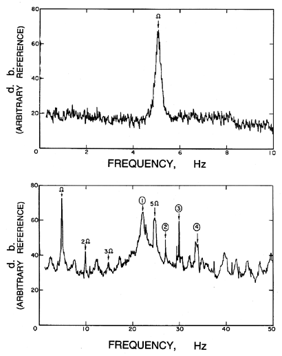
|
| Figure 8.1 Typical spectra of vibration for a centrifugal pump (Impeller X/Volute A) operating at 300rpm (Chamieh et al. 1985). |
Before proceeding to a discussion of the specific vibrational problems outlined above, it may be valuable to illustrate the spectral content of the shaft vibration of a typical centrifugal pump in normal, nominally steady operation. Figure 8.1 presents examples of the spectra (for two frequency ranges) taken from the shaft of the five-bladed centrifugal Impeller X operating in the vaneless Volute A (no stator blades) at 300rpm (5Hz). Clearly the synchronous vibration at the shaft fundamental of 5Hz dominates the low frequencies; this excitation may be caused by mechanical imperfections in the shaft such as an imbalance or by circumferential nonuniformities in the flow such as might be generated by the volute. It is also clear that the most dominant harmonic of shaft frequency occurs at 5Ω because there are 5 impeller blades. Note, however, that there are noticeable peaks at 2Ω and 3Ω arising from significantly nonsinusoidal excitation at the shaft frequency, Ω. The other dominant peaks labelled 1→ 4 represent structural resonant frequencies unaffected by shaft rotational speed.
|
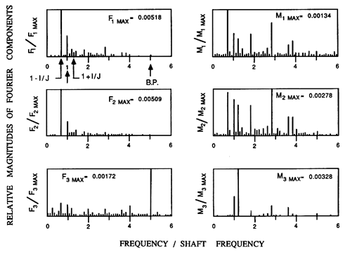
| Figure 8.2 Typical frequency content of F1, F2, F3, M1, M2, M3 for Impeller X/Volute A for tests at 3000 rpm, φ=0.092, and I/J=3/10. Note the harmonics Ω, (J± I)Ω/J and the blade passing frequency, 5Ω. |
At higher rotational speeds, more coincidence with structural frequencies occurs and the spectra contain more noise. However, interesting features can still be discerned. Figure 8.2 presents examples, taken from Miskovish and Brennen (1992), of the spectra for all six shaft forces and moments as measured in the rotating frame of Impeller X by the balance onto which that impeller was mounted. F1, F2 are the two rotating radial forces, M1, M2 are the corresponding bending moments, F3 is the thrust and M3 is the torque. In this example, the shaft speed is 3000rpm (Ω=100π rad/sec) and the impeller is also being whirled at a frequency, ω=IΩ/J, where I/J=3/10. Note that there is a strong peak in all the forces and moments at the shaft frequency, Ω, because of the steady radial forces caused by volute asymmetry. Rotordynamic forces would be manifest in this rotating frame at the beat frequencies (J± I)Ω/J; note that the predominant rotordynamic effect occurs at the lower of these beat frequencies, (J-I)Ω/J. The moments M1 and M2 are noisy because the line of action of the forces F1 and F2 is close to the chosen axial location of the origin of the coordinate system, the mid-point of the impeller discharge. Consequently, the magnitudes of the moments are small. One of the more surprising features in this data is the fact that the unsteady thrust contains a significant component at the blade passing frequency, 5Ω. Miskovish and Brennen (1992) indicate that the magnitude of this unsteady thrust is about 0.2→ 0.5% of the steady thrust and that the peaks occur close to the times when blades pass the volute cutwater. While this magnitude may not seem large, it could give rise to significant axial vibration at the blade passing frequency in some applications.
8.3 UNSTEADY FLOWS
Many of the phenomena listed in section 8.1 require some knowledge of the unsteady flows corresponding to the steady cascade flows discussed in sections 3.2 and 3.5. In the case of non-cavitating axial cascades, a large volume of literature has been generated in the context of gas turbine engines, and there exist a number of extensive reviews including those by Woods (1961), McCroskey (1977), Mikolajczak et al. (1975) and Platzer (1978). Much of the analytical work utilizes linear cascade theory, for example, Kemp and Sears (1955), Woods (1955), Schorr and Reddy (1971), and Kemp and Ohashi (1975). Some of this has been applied to the analysis of unsteady flows in pumps and extended to cover the case of radial or mixed flow machines. For example, Tsukamoto and Ohashi (1982) utilized these methods to model the start-up transients in centifugal pumps and Tsujimoto et al. (1986) extended the analysis to evaluate the unsteady torque in mixed flow machines.
However, most of the available methods are restricted to lightly loaded cascades and impellers at low angles of incidence. Other, more complex, theories (for example, Adamczyk 1975) are needed at larger angles of incidence and for highly cambered cascades when there is a strong coupling between the steady and unsteady flow (Platzer 1978). Moreover, most of the early theories were only applicable to globally uniform unsteady flows in which the blades all move in unison. Samoylovich (1962) appears to have been the first to consider oscillations with arbitrary interblade phase differences, the kind of analysis needed for flutter investigations (see below).
When the incidence angles are large so that the blades stall, one must resort to unsteady free streamline methods in order to model the flows (Woods 1961). Apart from the work of Sisto (1967), very little analytical work has been done on this problem which is of considerable importance in the context of turbomachinery. One of the fluid mechanical complexities is the unsteady or dynamic response of a separated flow that may lead to significant departures from the sucession of events one might construct based on a quasistatic approach. Some progress has been made in understanding the ``dynamic stall'' for a single foil (see, for example, Ham 1968). However, it would appear that more work is needed to understand the complex dynamic stall phenomena in turbomachines.
|
Figure 8.3
Fluctuating lift coefficient,  ,
for foils undergoing
heave oscillations at a reduced frequency, ω*=ω c/U.
Real and imaginary parts of
/ω* are presented for
(a) non-cavitating flow at mean incidence angles of 0° and 6°
(b) cavitating data for a mean incidence of 8°, for very long
choked cavities (squares) and for cavities 3 chords in length (diamonds).
Adapted from Acosta and DeLong (1971). ,
for foils undergoing
heave oscillations at a reduced frequency, ω*=ω c/U.
Real and imaginary parts of
/ω* are presented for
(a) non-cavitating flow at mean incidence angles of 0° and 6°
(b) cavitating data for a mean incidence of 8°, for very long
choked cavities (squares) and for cavities 3 chords in length (diamonds).
Adapted from Acosta and DeLong (1971).
|
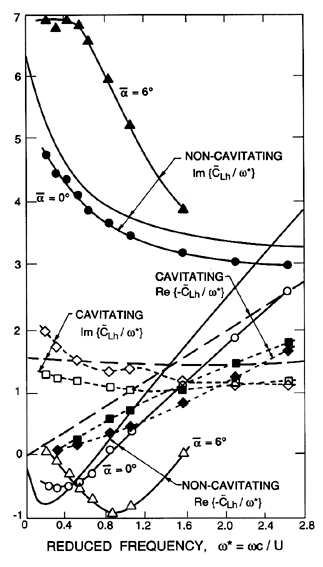
Unsteady free streamline analyses can be more confidentally applied to the analysis of cavitating cascades because the cavity or free streamline pressure is usually known and constant whereas the corresponding pressure for the wake flows may be varying with time in a way that is difficult to predict. Thus, for example, the unsteady response for a single supercavitating foil (Woods 1957, Martin 1962, Parkin 1962) has been compared with experimental measurements by Acosta and DeLong (1971). As an example, we present (figure 8.3) some data from Acosta and DeLong on the unsteady forces on a single foil undergoing heave oscillations at various reduced frequencies, ω*=ω c/2U. The oscillating heave motion, d, is represented by
 | ......(8.1) |
 , contains the amplitude and phase
of the displacement. The resulting lift coefficient,
CL, is decomposed
(using the notation of the next chapter) into
, contains the amplitude and phase
of the displacement. The resulting lift coefficient,
CL, is decomposed
(using the notation of the next chapter) into
 | ......(8.2) |
/ω* which are
plotted in figure 8.3 represent the unsteady lift characteristics
of the foil.
It is particularly important to note that substantial departures from
quasistatic behaviour occur for reduced frequencies as low as 0.2,
though these departures are more significant in the noncavitating flow
than in the cavitating flow.
The lines without points in figure 8.3 present results for the
corresponding linear theories and we observe that the agreement between
the theory and the experiments is fairly good.
Notice also that the
Re{-} for noncavitating foils
is negative at low frequencies but becomes
positive at larger ω whereas the values in the cavitating case are
all positive.
Similar data for cavitating cascades would be necessary in order to
analyse the potential for instability in cavitating, axial flow pumps.
The author is not aware of any such data or analysis.
The information is similarly meagre for all of the corresponding dynamic characteristics of radial rather than axial cascades and, consequently, our ability to model dynamic instabilities in centrifugal pumps is very limited indeed.
8.4 ROTATING STALL
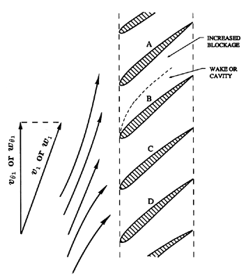
Rotating stall is a phenomenon which may occur in a cascade of blades when these are required to operate at a high angle of incidence close to that at which the blades will stall. In a pump this usually implies that the flow rate has been reduced to a point close to or below the maximum in the head characteristic (see, for example, figures 7.5 and 7.6). Emmons et al. (1955) first provided a coherent explanation of propagating stall. The cascade in figure 8.4 will represent a set of blades (a rotor or a stator) operating at a high angle of incidence. Then, if blade B were stalled, this generates a separated wake and therefore increased blockage to the flow in the passage between blades B and A. This, in turn, would tend to deflect the flow away from this blockage in the manner indicated in the figure. The result would be an increase in the angle of incidence on blade A and a decrease in the angle of incidence on blade C. Thus, blade A would tend to stall while any stall on blade C would tend to diminish. Consequently, the stall ``cell'' would tend to move upwards in the figure or in a direction away from the oncoming flow. Of course, the stall cell could consist of a larger number of blades with more than one exhibiting increased separation or stall. The stall cell will rotate around the axis and hence the name ``rotating stall.'' Moreover, the speed of propagation will clearly be some fraction of the circumferential component of the relative velocity, either vθ1 in the case of a stator or wθ1 in the case of a rotor. Consequently, in the case of a rotor, the stall rotates in the same direction as the rotor but with 50-70% of the rotor angular velocity.
|
| Figure 8.4 Schematic of a stall cell in rotating stall or rotating cavitation. |
In distinguishing between rotating stall and surge, it is important to note that the disturbance depicted in figure 8.4 does not necessarily imply any oscillation in the total mass flow rate through the turbomachine. Rather it implies a redistribution of that flow. On the other hand, it is always possible that the perturbation caused by rotating stall could resonate with, say, one of the acoustic modes in the inlet or discharge lines, in which case significant oscillation of the mass flow rate could occur.
While rotating stall can occur in any turbomachine, it is most frequently observed and most widely studied in compressors with large numbers of blades. Excellent reviews of this literature have been published by Emmons et al. (1959) and more recently by Greitzer (1981). Both point to a body of work designed to predict both the onset and consequences of rotating stall. A useful approximate criterion is that rotating stall in the rotor occurs when one approaches a maximum in the total head rise as the flow coefficient decreases. This is, however, no more than a crude approximation and Greitzer (1981) quotes a number of cases in which rotating stall occurs while the slope of the performance curve is still negative. A more sophisticated criterion that is widely used is due to Leiblein (1965), and involves the diffusion factor, Df, defined previously in equation 3.20. Experience indicates that rotating stall may begin when Df is increased to a value of about 0.6.
Though most of the observations of rotating stall have been made for axial compressors, Murai (1968) observed and investigated the phenomenon in a typical axial flow pump with 18 blades, a hub/tip radius ratio of 0.7, a tip solidity of 1.15, and a tip blade angle of 20°. His data on the rotating speed of the stall cell are reproduced in figure 8.5. Note that the onset of the rotating stall phenomenon occurs when the flow rate is reduced to a point below the maximum in the head characteristic. Notice also that the stall cell propagation velocities have typical values between 0.45 and 0.6 of the rotating speed.
|
| Figure 8.5 The head characteristic for an 18-bladed axial flow pump along with the measurements of the propagation velocity of the rotating stall cell relative to the shaft speed. Adapted from Murai (1968). Data is shown for three different inlet pressures. Flow and head scales are dimensionless. |
Rotating stall has not, however, been reported in pumps with a small number of blades perhaps because Df will not approach 0.6 for typical axial pumps or inducers with a small number of blades. Most of the stability theories (for example, Emmons et al. 1959) are based on actuator disc models of the rotor in which it is assumed that the stall cell is much longer than the distance between the blades. Such an assumption would not be appropriate in an axial flow pump with three or four blades.
Murai (1968) also examined the effect of limited cavitation on the rotating stall phenomenon and observed that the cavitation did cause some alteration in the propagation speed as illustrated by the changes with inlet pressure seen in figure 8.5. It is, however, important to emphasize the difference between the phenomenon observed by Murai in which cavitation is secondary to the rotating stall and the phenomenon to be discussed below, namely rotating cavitation, which occurs at a point on the head-flow characteristic at which the slope is negative and stable, and at which rotating stall would not occur.
Turning now to centrifugal pumps, there have been a number of studies in which rotating stall has been observed either in the impeller or in the diffuser/volute. Hergt and Benner (1968) observed rotating stall in a vaned diffuser and conclude that it only occurs with some particular diffuser geometries. Lenneman and Howard (1970) examined the blade passage flow patterns associated with rotating stall and present data on the ratio, ΩRS/Ω, of the propagation velocity of the stall cell to the impeller speed, Ω. They observed ratios ranging from 0.54 to 0.68 with, typically, lower values of the ratio at lower impeller speeds and at higher flow coefficients.
Perhaps the most detailed study is the recent research of Yoshida et al. (1991) who made the following observations on a 7-bladed centrifugal impeller operating with a variety of diffusers, with and without vanes. Rotating stall with a single cell was observed to occur in the impeller below a certain critical flow coefficient which depended on the diffuser geometry. In the absence of a diffuser, the cell speed was about 80-90% of the impeller rotating speed; with diffuser vanes, this cell speed was reduced to the range 50-80%. When impeller rotating stall was present, they also detected the presence of some propagating disturbances with 2, 3 and 4 cells rather than one. These are probably due to nonlinearities and an interaction with blade passage excitation. Rotating stall was also observed to occur in the vaned diffuser with a speed less than 10% of the impeller speed. It was most evident when the clearance between the impeller and diffuser vanes was large. As this clearance was decreased, the diffuser rotating stall tended to disappear.
Even in the absence of blades, it is possible for a diffuser or volute to exhibit a propagating rotating ``stall''. Jansen (1964) and van der Braembussche (1982) first described this flow instability and indicate that the flow pattern propagates with a speed in the range of 5-25% of the impeller speed. Yoshida et al. (1991) observed a four-cell rotating stall in their vaneless diffusers over a large range of flow coefficients and measured its velocity as about 20% of the impeller speed.
Finally, we note that rotating stall may resonate with an acoustic mode of the inlet or discharging piping to produce a serious pulsation problem. Dussourd (1968) identified such a problem in a boiler feed system in which the rotating stall frequency was in the range 0.15Ω→ 0.25Ω, much lower than usual. He also made use of the frequency domain methods of chapter 9 in modelling the dynamics of this multistage centrifugal pump system. This represents a good example of one of the many hybrid problems that can arise in systems with turbomachines.
Inducers or impellers in pumps that do not show any sign of rotating stall while operating under noncavitating conditions may exhibit a superficially similar phenemenon known as ``rotating cavitation'' when they are required to operate at low cavitation numbers. However, it is important to emphasize the fundamental difference in the two phenomena. Rotating stall occurs at locations along the head-flow characteristic at which the blades may stall, usually at flow rates for which the slope of the head/flow characteristic is positive and therefore unstable in the sense discussed in the next section. On the other hand, rotating cavitation is observed to occur at locations where the slope is negative. These would normally be considered stable operating points in the absence of cavitation. Consequently, the dynamics of the cavitation are essential to rotating cavitation. Another difference between the phenomena is the difference in the propagating speeds.
|
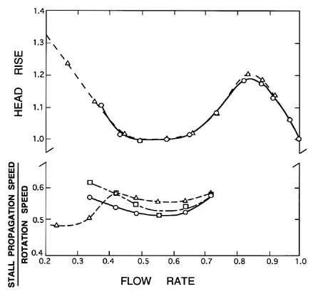
| Figure 8.6 Occurrence of rotating cavitation and auto-oscillation in the performance of the cavitating inducer tested by Kamijo et al. (1977). |
Rotating cavitation was first explicitly identified by Kamijo, Shimura and Watanabe (1977) (see also 1980), though some evidence of it can be seen in the shaft vibration measurements of Rosemann (1965). When it has been observed, rotating cavitation generally occurs when the cavitation number, σ, is reduced to a value at which the head is beginning to be affected by the cavitation as seen in figure 8.6 taken from Kamijo et al. (1977). Rosenmann (1965) reported that the vibrations (that we now recognize as rotating cavitation) occurred for cavitation numbers between 2 and 3 times the breakdown value and were particularly evident at the lower flow coefficients at which the inducer was more heavily loaded.
Usually, further reduction of σ below the value at which rotating cavitation occurs will lead to auto-oscillation or surge (see below and figure 8.6). It is not at all clear why some inducers and impellers do not exhibit rotating cavitation at all but proceed directly to auto-oscillation if that instability is going to occur.
Unlike rotating stall whose rotational velocities are less than that of the rotor, rotating cavitation is characterized by a propagating velocity that is slightly larger than the impeller speed. Kamijo et al. (1977) (see also Kamijo et al. 1992) observed propagating velocities ΩRC /Ω of about 1.15, and this is very similar to one of the somewhat ambigous propagating disturbance velocities of 1.1 Ω reported by Rosemann (1965).
Recently, Tsujimoto et al. (1992) have utilized the methods of chapter 9 to model the dynamics of rotating cavitation. They have shown that the cavitation compliance and mass flow gain factor (see section 9.14) play a crucial role in determining the instability of rotating cavitation in much the same way as these parameters influence the stability of an entire system which includes a cavitating pump (see section 8.7). Also note that the analysis of Tsujimoto et al. (1992) predicts supersynchronous propagating speeds in the range ΩRC/Ω= 1.1 to 1.4, consistent with the experimental observations.
8.6 SURGE
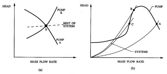
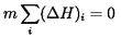
Surge and auto-oscillation (see next section) are system instabilities that involve not just the characteristics of the pump but those of the rest of the pumping system. They result in pressure and flow rate oscillations that can not only generate excessive vibration and reduce performance but also threaten the structural integrity of the turbomachine or other components of the system. In chapter 9 we provide more detail on general analytical approaches to this class of system instabilities. But for present purposes, it is useful to provide a brief outline of some of the characteristics of these system instabilities. To do so, consider first figure 8.7(a) in which the steady-state characteristic of the pump (head rise} versus mass flow rate) is plotted together with the steady-state characteristic of the rest of the system to which the pump is connected (head drop} versus mass flow rate). In steady-state operation the head rise across the pump must equal the head drop for the rest of the system, and the flow rates must be the same so that the combination will operate at the intersection, O. Consider, now, the response to a small decrease in the flow to a value just below this equilibrium point, O. Pump A will then produce more head than the head drop in the rest of the system, and this discrepancy will cause the flow rate to increase, causing a return to the equilibrium point. Therefore, because the slope of the characteristic of Pump A is less than the slope of the characteristic of the rest of the system, the point O represents a quasistatically stable operating point. On the other hand, the system with Pump B is quasistatically unstable. Perhaps the best known example of this kind of instability occurs in multistage compressors in which the characteristics generally take the shape shown in figure 8.7(b). It follows that the operating point A is stable, point B is neutrally stable, and point C is unstable. The result of the instability at points such as C is the oscillation in the pressure and flow rate known as ``compressor surge.''
|
| Figure 8.7 Quasistatically stable and unstable operation of pumping systems. |
While the above description of quasistatic stability may help in visualizing the phenomenon, it constitutes a rather artificial separation of the total system into a ``pump" and ``the rest of the system." A more general analytical perspective is obtained by defining a resistance, R*i, for each of the series components of the system (one of which would be the pump) distinguished by the subscript, i:
 | ......(8.3) |
 | ......(8.4) |
Perhaps the most satisfactory interpretation of the above formulation is in terms of the energy balance of the total system. The net flux of energy out of each of the elements of the system is m (ΔH)i. Consequently, the net energy flux out of the system is
 | ......(8.5) |
Suppose the stability of the system is now explored by inserting somewhere in the system a hypothetical perturbing device which causes an increase in the flow rate by dm. Then the new net energy flux out of the system, E*, is given by
 |
|
All of the above is predicated on the changes to the system being sufficiently slow for the pump and the system to follow the steady state operating curves. Thus the analysis is only applicable to those instabilities whose frequencies are low enough to lie within some quasistatic range. At higher frequency, it is necessary to include the inertia and compressibility of the various components of the flow. Greitzer (1976) (see also 1981) has developed such models for the prediction of both surge and rotating stall in axial flow compressors.
It is important to observe that, while quasisteady instabilities will certainly occur when the sum of all the R*i is less than zero, there may be other dynamic instabilities that occur even when the system is quasistatically stable. One way to view this possibility is to recognize that the resistance of any flow is frequently a complex function of frequency once a certain quasisteady frequency has been exceeded. Consequently, the resistances, R*i, may be different at frequencies above the quasistatic limit. It follows that there may be operating points at which the total dynamic resistance over some range of frequencies is negative. Then the system would be dynamically unstable even though it may still be quasistatically stable. Such a description of dynamic instability is instructive but overly simplistic and a more systematic approach to this issue must await the methodologies of chapter 9.
8.7 AUTO-OSCILLATION
|
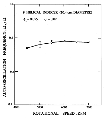
| Figure 8.8 Data from Braisted and Brennen (1980) on the ratio of the auto-oscillation frequency to the shaft frequency as a function of the latter for a 9° helical inducer operating at a cavitation number of 0.02 and a flow coefficient of 0.055. |
|
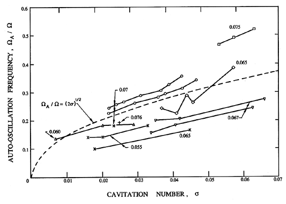
| Figure 8.9 Data from Braisted and Brennen (1980) on the ratio of the frequency of auto-oscillation to the frequency of shaft rotation for several inducers: SSME Low Pressure LOX Pump models: 7.62cm diameter operating at 9000rpm (×) and 12000rpm (+), 10.2cm diameter operating at 4000rpm (circles) and 6000rpm (squares); 9° helical inducers: 7.58cm diameter operating at 9000rpm *, 10.4cm diameter with suction line flow straightener (triangles upsidedown) and without suction line flow straightener (triangles). The flow coefficients, φ1, are as labelled. |
In many installations involving a pump that cavitates, violent oscillations in the pressure and flow rate in the entire system occur when the cavitation number is decreased to values at which the head rise across the pump begins to be affected (Braisted and Brennen 1980, Kamijo et al. 1977, Sack and Nottage 1965, Natanzon et al. 1974, Miller and Gross 1967, Hobson and Marshall 1979). These oscillations can also cause substantial radial forces on the shaft of the order of 20% of the axial thrust (Rosenmann 1965). This surge phenomenon is known as auto-oscillation and can lead to very large flow rate and pressure fluctuations in the system. In boiler feed systems, discharge pressure oscillations with amplitudes as high as 14bar have been reported informally. It is a genuinely dynamic instability in the sense described in the last section, for it occurs when the slope of the pump head rise/flow rate curve is still strongly negative. Another characteristic of auto-oscillation is that it appears to occur more readily when the inducer is more heavily loaded; in other words at lower flow coefficients. These are also the circumstances under which backflow will occur. Indeed, Badowski (1969) puts forward the hypothesis that the dynamics of the backflow are responsible for cavitating inducer instability. Further evidence of this connection is provided by Hartmann and Soltis (1960) but with an atypical inducer that has 19 blades. It is certainly the case that the limit cycle associated with a strong auto-oscillation appears to involve large periodic oscillations in the backflow. Consequently, it would seem that any nonlinear model purporting to predict the magnitude of auto-oscillation should incorporate the dynamics of the backflow. While most of the detailed investigations have focussed on axial pumps and inducers, Yamamoto (1991) has observed and investigated auto-oscillation occurring in cavitating centrifugal pumps. He also noted the important role played by the backflow in the dynamics of the auto-oscillation.
Unlike compressor surge, the frequency of auto-oscillation, ΩA, usually scales with the shaft speed of the pump. Figure 8.8 demonstrates this by plotting ΩA/Ω against the shaft rpm (60Ω/2π) for a particular helical inducer. Figure 8.9 (also from Braisted and Brennen 1980) shows how this reduced auto-oscillation frequency, ΩA/Ω, varies with flow coefficient, φ, cavitation number, σ, and impeller geometry. While still noting that the frequency, ΩA, will, in general, be system dependent, nevertheless the expression
 | ......(8.8) |
|
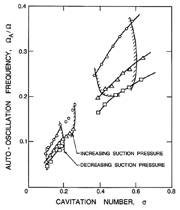
| Figure 8.10 Data from Yamamoto (1991) on the ratio of the frequency of auto-oscillation to the frequency of shaft rotation for a centrifugal pump. Data is shown for three different lengths of suction pipe: 2.7m (circles), 4.9m (upsidedown triangles) and 7.1m (squares). Regions of instability are indicated by the hatched lines. |
Some data from Yamamoto (1991) on the frequencies of auto-oscillation of a cavitating centrifugal pump are presented in figure 8.10. This data exhibits a dependence on the length of the suction pipe that reinforces the understanding of auto-oscillation as a system instability. The figure also shows the limits of instability observed by Yamamoto; these are unusual in that there appear to be two separate regions or zones of instability. Finally, it is clear that the data of figures 8.9 and 8.10 show a similar dependence of the auto-oscillation frequency on the cavitation number, σ, though the magnitudes of σ differ considerably. However, it is likely that the relative sizes of the cavities are similiar in the two cases, and therefore that the correlation between the auto-oscillation frequency and the relative cavity size might be closer than the correlation with cavitation number.
As previously stated, auto-oscillation occurs when the region of cavitation head loss is approached as the cavitation number is decreased. Figure 8.11 provides an example of the limits of auto-oscillation taken from the work of Braisted and Brennen (1980). However, since the onset is even more dependent than the auto-oscillation frequency on the detailed dynamic characteristics of the system, it would not even be wise to quote any approximate guideline for onset. Our current understanding is that the methodologies of chapter 9 are essential for any prediction of auto-oscillation.
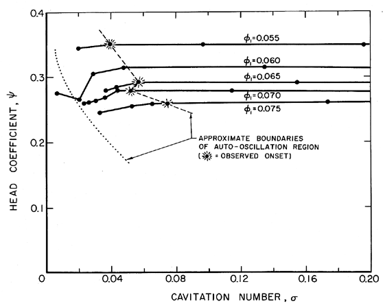
|
| Figure 8.11 Cavitation performance of the SSME low pressure LOX pump model, Impeller IV, showing the onset and approximate desinence of the auto-oscillation at 6000rpm (from Braisted and Brennen 1980). |
|
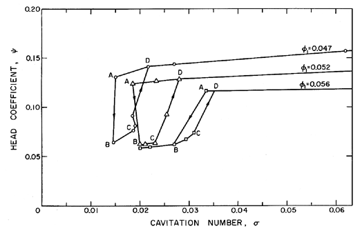
| Figure 8.12 Data from a helical inducer illustrating the decrease in head with the onset of auto-oscillation (A→ B) and the auto-oscillation hysteresis occurring with subsequent increase in σ (from Braisted and Brennen 1980). |
It should be noted that chapter 9 describes linear perturbation models that can predict the limits of oscillation but not the amplitude of the oscillation once it occurs. There do not appear to be any accepted analytical models that can make this important prediction. Furthermore, the energy dissipated in the large amplitude oscillations within the pump can lead to a major change in the mean (time averaged) performance of the pump. One example of the effect of auto-oscillation on the head rise across a cavitating inducer is shown in figure 8.12 (from Braisted and Brennen 1980) which contains cavitation performance curves for three flow coefficients. The sequence of events leading to these results was as follows. For each flow rate, the cavitation number was decreased until the onset of auto-oscillation at the point labelled A, when the head immediately dropped to the point B (an unavoidable change in the pump inlet pressure and therefore in σ would often occur at the same time). Increasing the cavitation number again would not immediately eliminate the auto-oscillation. Instead the oscillations would persist until the cavitation number was raised to the value at the point C where the disappearance of auto-oscillation would cause recovery to the point D. This set of experiments demonstrate (i) that under auto-oscillation conditions (B,C) the head rise across this particular inducer was about half of the head rise without auto-oscillation (A,D) and (ii) that a significant auto-oscillation hysteresis exists in which the auto-oscillation inception and desinence cavitation numbers can be significantly different. Neither of these nonlinear effects can be predicted by the frequency domain methods of chapter 9. In other inducers, the drop in head with the onset of auto-oscillation is not as large as in figure 8.12 but it is still present; it has also been reported by Rosenmann (1965). This effect may account for the somewhat jagged form of the cavitation characteristic as breakdown is approached.
8.8 ROTOR-STATOR INTERACTION: FLOW PATTERNS
In section 8.2, we described the two basic frequencies of rotor-stator interaction: the excitation of the stator flow at ZRΩ and the excitation of the rotor flow at ZSΩ. Apart from the superharmonics mZRΩ and mZSΩ that are generated by nonlinearities, subharmonics can also occur. When they do they can cause major problems, since the fluid and structural damping is smaller for these lower frequencies. To avoid such subharmonics, turbomachines are usually designed with blade numbers, ZR and ZS, which have small integer common factors.
|
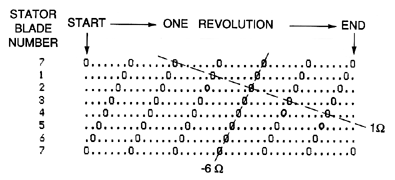
| Figure 8.13 Encounter diagram for rotor-stator interaction in a turbomachine with ZR=6, ZS=7. Each row is for a specific stator blade and time runs horizontally covering one revolution as one proceeds from left to right. Encounters between a rotor blade and a stator blade are marked by an 0. |
|
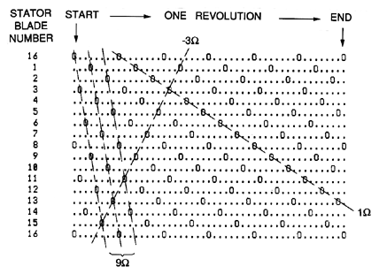
| Figure 8.14 Encounter diagram for rotor-stator interaction in a turbomachine with ZR=6, ZS=16. |
|
| Figure 8.15 The propagation of a low pressure region (hatched) at nine times the impeller rotational speed in the flow through a high head pump-turbine. The sketches show six instants in time equally spaced within one sixth of a revolution. Made from videotape provided by Miyagawa et al. (1992). |
The various harmonics of blade passage excitation can be visualized by generating an ``encounter'' (or interference) diagram that is a function only of the integers ZR and ZS. In these encounter diagrams, of which figures 8.13 and 8.14 are examples, each of the horizontal lines represents the position of a particular stator blade. The circular geometry has been unwrapped so that a passing rotor blade proceeds from top to bottom as it rotates past the stator blades. Each vertical line represents a moment in time, the period covered being one complete revolution of the rotor beginning at the far left and returning to that moment on the far right. Within this framework, the moment and position of all the rotor-stator blade encounters are shown by an ``0.'' Such encounter diagrams allow one to examine the various frequencies and patterns generated by rotor-stator interactions and this is perhaps best illustrated by referring to the examples of figure 8.13 for the case of ZR=6, ZS=7, and figure 8.14 for the case of ZR=6, ZS=16. First, one can always follow the diagonal progress of individual rotor blades as indicated by lines such as those marked 1Ω in the examples. But other diagonal lines are also evident. For example, in figure 8.13 the perturbation consisting of a single cell, and propagating in the reverse direction at 6Ω is strongly indicated. Parenthetically we note that, in any machine in which ZS=ZR+1, a perturbation with a reverse speed of -ZRΩ is always present. Also in figure 8.14, there are quite strong lines indicating an encounter pattern rotating at 9Ω and consisting of two diametrically opposite cells. Other propagating disturbance patterns are also suggested by figure 8.14. For example, the backward propagating disturbance rotating at 3Ω in the reverse direction and consisting of four equally spaced perturbation cells is indicated by the lines marked -3Ω. It is, of course, possible to connect up the encounter points in a very large number of ways, but clearly only those disturbances with a large number of encounters per cycle (high ``density'') will generate a large enough flow perturbation to be significant. However, among the top two or three possibilities, it is not necessarily a simple matter to determine which will manifest itself in the actual flow. That requires more detailed analysis of the flow.
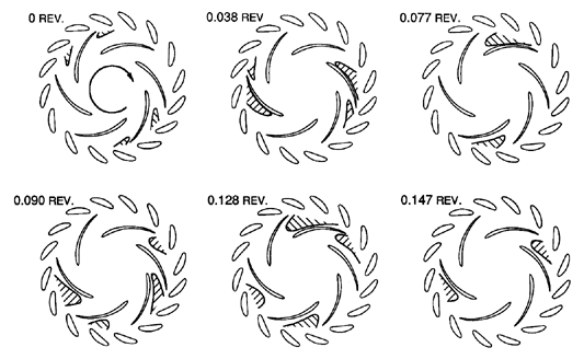
The flow perturbations caused by blade passage excitation are nicely illustrated by Miyagawa et al. (1992) in their observations of the flows in high head pump turbines. One of the cases they explored was that of figure 8.14, namely ZR=6, ZS=16. Figure 8.15 has been extracted from the videotape of their unsteady flow observations and shows two diametrically opposite perturbation cells propagating around at 9 times the impeller rotating speed, one of the ``dense'' perturbation patterns predicted by the encounter diagram of figure 8.14.
8.9 ROTOR-STATOR INTERACTION: FORCES
When one rotor (or stator) blade passes through the wake of an upstream stator (or rotor) blade, it will clearly experience a fluctuation in the fluid forces that act upon it. In this section, the nature and magnitude of these rotor-stator interaction forces will be explored. Experience has shown that these unsteady forces are a strong function of the gap between the locus of the trailing edge of the upstream blade and the locus of the leading edge of the downstream blade. This distance will be termed the interblade spacing, and will be denoted by cb.
|
| Figure 8.16 Pressure distributions on a diffuser blade at two different instants during the passage of an impeller blade. Data for an interblade spacing of 1.5% and φ2=0.12 (from Arndt et al. 1989). |
Most axial compressors and turbines operate with fairly large interblade spacings, greater than 10% of the blade chord. As a result, the unsteady flows and forces measured under these circumstances (Gallus 1979, Gallus et al. 1980, Dring et al. 1982, Iino and Kasai 1985) are substantially smaller than those measured for radial machines (such as centrifugal pumps) in which the interblade spacing between the impeller and diffuser blades may be only a few percent of the impeller radius. Indeed, structural failure of the leading edge of centrifugal diffuser blades is not uncommon in the industry, and is typically solved by increasing the interblade spacing, though at the cost of reduced hydraulic performance.
Several early investigations of rotor-stator interaction forces were carried out using single foils in a wind tunnel (for example, Lefcort 1965). However, Gallus et al. (1980) appear to have been the first to measure the unsteady flows and forces due to rotor-stator interaction in an axial flow compressor. They attempt to collate their measurements with the theoretical analyses of Kemp and Sears (1955), Meyer (1958), Horlock (1968) and others. The measurements were conducted with large interblade spacing to axial chord ratios of about 50%, and involved documentation of the blade wakes. The impingement of these wakes on the following row of blades causes pressure fluctuations that are largest on the forward suction surface and small near the trailing edge of those blades. These pressure fluctuations lead to a fluctuation in the lift coefficient of ± 0.06. Moreover, Gallus et al. (1980) show that the forces vary roughly inversely with the interblade spacing to axial chord ratio. Extrapolation would suggest that the unsteady and steady components of the lift might be roughly the same if this ratio were decreased to 5%. This estimate is confirmed by the measurements of Arndt et al., described below. Before concluding this discussion of rotor-stator interaction forces in axial flow machines, we note that Dring et al. (1982) have examined the flows and forces for an interblade spacing to axial chord ratio of 0.35 and obtained results similar to those of Gallus et al..
|
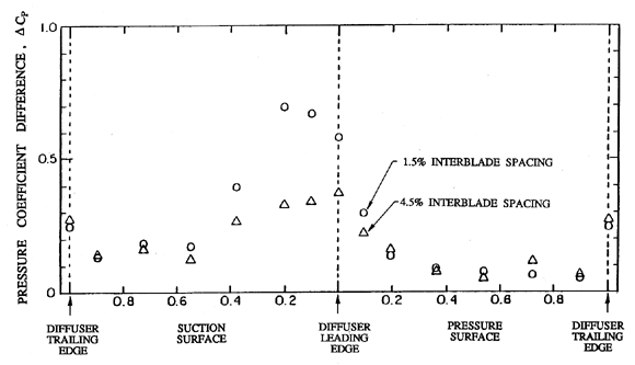
| Figure 8.17 Magnitude of the fluctuation in the coefficient of pressure on a diffuser blade during the passage of an impeller blade as a function of location on the diffuser blade surface for two interblade spacings (from Arndt et al. 1989). |
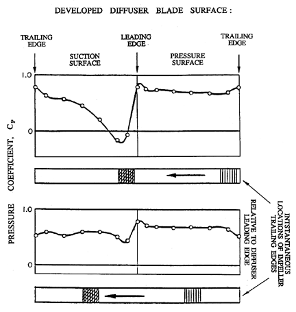
Recently, Arndt et al. (1989, 1990) (see also Brennen et al. 1988) have made measurements of the unsteady pressures and forces that occur in a radial flow machine when an impeller blade passes a diffuser blade. Figure 8.16 presents instantaneous pressure distributions (ensemble-averaged over many revolutions) for two particular relative positions of the impeller and diffuser blades. In the upper graph the trailing edge of the impeller blade has just passed the leading edge of the diffuser blade, causing a large perturbation in the pressure on the suction surface of the diffuser blade. Indeed, in this example, the pressure over a small region has fallen below the impeller inlet pressure (Cp<0). The lower graph is the pressure distribution at a later time when the impeller blade is about half-way to the next diffuser blade. The perturbation in the diffuser blade pressure distribution has largely dissipated. Closer examination of the data suggests that the perturbation takes the form of a wave of negative pressure traveling along the suction surface of the diffuser blade and being attenuated as it propagates. This and other observations suggest that the cause is a vortex shed from the leading edge of the diffuser blade by the passage of the trailing edge of the impeller. This vortex is then convected along the suction surface of the diffuser blade.
|
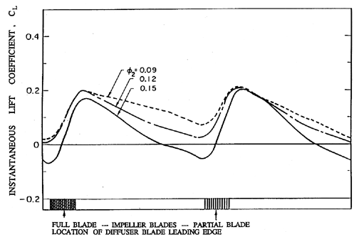
| Figure 8.18 Variation in the instantaneous lift coefficient for a diffuser blade. The position of the diffuser blade leading edge relative to the impeller blade trailing edge is also shown. The data is for an interblade spacing of 4.5% (from Arndt et al. 1989). |
The difference between the maximum and minimum pressure coefficient, ΔCp, experienced at each position on the surface of a diffuser blade is plotted as a function of position in figure 8.17. Data is shown for two interblade spacings, cb=0.015 RT2 and 0.045 RT2. This figure reiterates the fact that the pressure perturbations are largest on the suction surface just downstream of the leading edge. It also demonstrates that the pressure perturbations for the 1.5% interblade spacing are about double those for the 4.5% interblade spacing. Figure 8.17 was obtained at a particular flow coefficient of φ2=0.12; however, the same phenomena were encountered in the range 0.05<φ2<0.15, and the magnitude of the pressure perturbation showed an increase of about 50% between φ2= 0.05 and φ2=0.15.
|
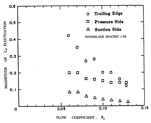
| Figure 8.19 Magnitude of the fluctuations in the pressure coefficient at three locations near the trailing edge of an impeller blade during the passage of a diffuser blade (from Arndt et al. 1990). |
Given both the magnitude and phase of the instantaneous pressures on the surface of a diffuser blade, the result may be integrated to obtain the instantaneous lift, L, on the diffuser blade. Here the lift coefficient is defined as CL=L/½ρΩ2 R2T2cb where L is the force on the blade perpendicular to the mean chord, c is the chord, and b is the span of the diffuser blade. Time histories of CL are plotted in figure 8.18 for three different flow coefficients and an interblade spacing of 4.5%. Since the impeller blades consisted of main blades separated by partial blades, two ensemble-averaged cycles are shown for CL though the differences between the passage of a full blade and a partial blade are small. Notice that even for the larger 4.5% interblade spacing, the instantaneous lift can be as much as three times the mean lift. Consequently, a structural design criterion based on the mean lift on the blades would be seriously flawed. Indeed, in this case it is clear that the principal structural consideration should be the unsteady lift, not the steady lift.
Arndt et al. (1990) also examined the unsteady pressures on the upstream impeller blades for a variety of diffusers. Again, large pressure fluctuations were encountered as a result of rotor-stator interaction. Typical results are shown in figure 8.19 where the magnitude of the pressure fluctuations is presented as a function of flow coefficient for three different locations on the surface of an impeller blade: (i) on the flat of the trailing edge, (ii) on the suction surface at r/RT2 =0.937, and (iii) on the pressure surface at r/RT2=0.987. The data are for a 5% interblade spacing and all data points represent ensemble averages. The magnitudes of the fluctuations are of the same order as the pressure fluctuations on the diffuser blades, indicating that the unsteady loads on the upstream} blade in rotor-stator interaction can also be substantial. Note, however, that contrary to the trend with the diffuser blades, the magnitude of the pressure fluctuations decrease} with increasing flow coefficient. Finally, note that the magnitude of the pressure fluctuations are as large as the total head rise across the pump. This raises the possibility of transient cavitation being caused by rotor-stator interaction.
Considering the magnitude of these rotor-stator interaction effects, it is surprising that there is such a limited quantity of data available on the unsteady forces.
8.10 DEVELOPED CAVITY OSCILLATION
There are several circumstances in which developed cavities can exhibit self-sustained oscillations in the absence of any external excitation. One of these is the instability associated with a partial cavity whose length is approximately equal to the chord of the foil. Experimentally, it is observed that when the cavitation number is decreased to the level at which the attached partial cavity on a single hydrofoil approaches about 0.7 of the chord, c, of the foil, the cavity will begin to oscillate violently (Wade and Acosta 1966). It will grow to a length of about 1.5c, at which point the cavity will be pinched off at about 0.5c, and the separated cloud will collapse as it is convected downstream. This collapsing cloud of bubbles carries with it shed vorticity, so that the lift on the foil oscillates at the same time. This phenomenon is called ``partial cavitation oscillation.'' It persists with further decrease in cavitation number until a point is reached at which the cavity collapses at some critical distance downstream of the trailing edge that is usually about 0.3c. For cavitation numbers lower than this, the flow again becomes quite stable. The frequency of partial cavitation oscillation on a single foil is usually less than 0.1 U/c, where U is the velocity of the oncoming stream, and c is the chord length of the foil. In cascades or pumps, supercavitation is usually only approached in machines of low solidity, but, under such circumstances, partial cavitation oscillation can occur, and can be quite violent. Wade and Acosta (1966) were the first to observe partial cavitation oscillation in a cascade. During another set of experiments on cavitating cascades, Young, Murphy, and Reddcliff (1972) observed only ``random unsteadiness of the cavities.''
|
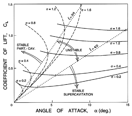
| Figure 8.20 The lift coefficient for a flat plate from the partial cavitation analysis of Acosta (1955) (dashed lines) and the supercavitating analysis of Tulin (1953) (solid lines); CL is shown as a function of angle of attack, α, for several cavitation numbers, σ. The dotted lines are the boundaries of the region in which the cavity length is between 3/4 and 4/3 of a chord, and in which dCL/dα<0. |
One plausible explanation for this partial cavitation instability can be gleaned from the free streamline solutions for a cavitating foil that were described in section 7.8. The results from equations 7.9 to 7.12 can be used to plot the lift coefficient as a function of angle of attack for various cavitation numbers, as shown in figure 8.20. The results from both the partial cavitation and the supercavitation analyses are shown. Moreover, we have marked with a dotted line the locus of those points at which the supercavitating solution yields dCL/dα=0; it is easily shown that this occurs when ℓ=4c/3. We have also marked with a dotted line the locus of those points at which the partial cavitation solution yields dCL/dα=∞; it can also be shown that this occurs when ℓ=3c/4. Note that these dotted lines separate regions for which dCL/dα>0 from that region in which dCL/dα<0. Heuristically, it could be argued that dCL/dα<0 implies an unstable flow. It would follow that the region between the dotted lines in figure 8.20 represents a regime of unstable operation. The boundaries of this regime are 3/4<ℓ/c<4/3, and do, indeed, seem to correspond quite closely to the observed regime of unstable cavity oscillation (Wade and Acosta 1966).
A second circumstance in which a fully developed cavity may exhibit natural oscillations occurs when the cavity is formed by introducing air to the wake of a foil in order to form a ``ventilated cavity.'' When the flow rate of air exceeds a certain critical level, the cavity may begin to oscillate, large pockets of air being shed at the rear of the main cavity during each cycle of oscillation. This problem was studied by Silberman and Song (1961) and by Song (1962). The typical radian frequency for these oscillations is about 6 U/ℓ, based on the length of the cavity, ℓ. Clearly, this second phenomenon is less relevant to pump applications.
8.11 ACOUSTIC RESONANCES
In the absence of cavitation or flow-induced vibration, flow noise generated within the turbomachine itself is almost never an issue when the fluid is a liquid. One reason for this is that the large wavelength of the sound in the liquid leads to internal acoustic resonances that are too high in frequency and, therefore, too highly damped to be important. This contrasts with the important role played by internal resonances in the production of noise in gas turbines and compressors (Tyler and Sofrin 1962, Cumpsty 1977). In noncavitating liquid turbomachinery, the higher acoustic velocity and the smaller acoustic damping mean that pipeline resonances play the same kind of role that the internal resonances play in the production of noise in gas turbomachinery.
In liquid turbomachines, resonances exterior to the machine or resonances associated with cavitation do create a number of serious vibration problems. As mentioned in the introduction, pipeline resonances with the acoustic modes of the inlet or discharge piping can occur when one of the excitation frequencies produced by the pump or hydraulic turbine happens to coincide with one of the acoustic modes of those pipelines. Jaeger (1963) and Strub (1963) document a number of cases of resonance in hydropower systems. Many of these do not involve excitation from the turbine but some do involve excitation at blade passing frequencies (Strub 1963). One of the striking features of these phenomena is that very high harmonics of the pipelines can be involved (20th harmonics have been noted) so that damage occurs at a whole series of nodes equally spaced along the pipeline. The cases described by Jaeger involve very large pressure oscillations, some of which led to major failures of the installation. Sparks and Wachel (1976) have similarly documented a number of cases of pipeline resonance in pumping systems. They correctly identify some of these as system instabilities of the kind discussed in section 8.6 and in chapter 9.
Cavitation-induced resonances and vibration problems are dealt with in other sections of this chapter. But it is appropriate in the context of resonances to mention one other possible cavitation mechanism even though it has not, as yet, been demonstrated experimentally. One might judge that the natural frequency, ωP, of bubbles given by equation 6.14 (section 6.5), being of the order of kHz, would be too high to cause vibration problems. However, it transpires that a finite cloud of bubbles may have much smaller natural frequencies that could resonant, for example, with a blade passage frequency to produce a problem. d'Agostino and Brennen (1983) showed that the lowest natural frequency, ωC, of a spherical cloud of bubbles of radius, A, consisting of bubbles of radius, R, and with a void fraction of α would be given by
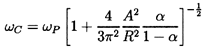 | ......(8.9) |
8.12 BLADE FLUTTER
Up to this point, all of the instabilities have been essentially hydrodynamic and would occur with a completely rigid structure. However, it needs to be observed that structural flexibility could modify any of the phenomena described. Furthermore, if a hydrodynamic instability frequency happens to coincide with the frequency of a major mode of vibration of the structure, the result will be a much more dangerous vibration problem. Though the hydroelastic behavior of single hydrofoils has been fairly well established (see the review by Abramson 1969), it would be virtually impossible to classify all of the possible fluid-structure interactions in a turbomachine given the number of possible hydrodynamic instabilities and the complexity of the typical pump structure. Rather, we shall confine attention to one of the simpler interactions and briefly discuss blade flutter. Though the rotor-stator interaction effects outlined above are more likely to cause serious blade vibration problems in turbomachines, it is also true that a blade may flutter and fail even in the absence of such excitation.
It is well known (see, for example, Fung 1955) that the incompressible, unstalled flow around a single airfoil will not exhibit flutter when permitted only one degree of freedom of flutter motion. Thus, classic aircraft wing flutter requires the coupling of two degrees of flutter motion, normally the bending and torsional modes of the cantilevered wing. Turbomachinery flutter is quite different from classic aircraft wing flutter and usually involves the excitation of a single structural mode. Several different phenomena can lead to single degree of freedom flutter when it would not otherwise occur in incompressible, unseparated (unstalled) flow. First, there are the effects of compressibility that can lead to phenomena such as supersonic flutter and choke flutter. These have been the subject of much research (see, for example, the reviews of Mikolajczak et al. (1975), Platzer (1978), Sisto (1977), McCroskey (1977)), but are not of direct concern in the context of liquid turbomachinery, though the compressibility introduced by cavitation might provide some useful analogies. Of greater importance in the context of liquid turbomachinery is the phenomenon of stall flutter (see, for example, Sisto 1953, Fung 1955). A blade which is stalled during all or part of a cycle of oscillation can exhibit single degree of freedom flutter, and this type of flutter has been recognized as a problem in turbomachinery for many years (Platzer 1978, Sisto 1977). Unfortunately, there has been relatively little analytical work on stall flutter and any modern theory must at least consider the characteristics of dynamic stall (see McCroskey 1977). Like all single degree of freedom flutter problems, including those in turbomachines, the critical incident speed for the onset of stall flutter, UC, is normally given by a particular value of a reduced speed, UCR=2 UC/c ωF, where c is the chord length and ωF is the frequency of flutter or the natural frequency of the participating structural vibration mode. The inverse of UCR is the reduced frequency, kCR, or Strouhal number. Fung (1955) points out that the reduced frequency for stall flutter with a single foil is a function of the difference, θ, between the mean angle of incidence of the flow and the static angle of stall. A crude guide would be kCR=0.3+4.5θ for 0.1<kCR<0.8. The second term in the expression for kCR reflects the decrease in the critical speed with increasing incidence.
Of course, in a turbomachine or cascade, the vibration of one blade will generate forces on the neighboring blades (see, for example, Whitehead 1960), and these interactions can cause significant differences in the flutter analyses and critical speeds; often they have a large unfavorable effect on the flutter characteristics (McCroskey 1977). One must allow for various phase angles between neighboring blades, and examine waves which travel both forward and backward relative to the rotation of the rotor. A complete analysis of the vibrational modes of the rotor (or stator) must be combined with an unsteady fluid flow analysis (see, for example, Verdon 1985) in order to accurately predict the flutter boundaries in a turbomachine. Of course, most of the literature deals with structures that are typical of compressors and turbines. The lowest modes of vibration in a pump, on the other hand, can be very different in character from those in a compressor or turbine. Usually the blades have a much smaller aspect ratio so that the lowest modes involve localized vibration of the leading or trailing edges of the blades. Consequently, any potential flutter is likely to cause failure of portions of these leading or trailing edges.
 <
< |
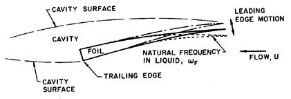
| Figure 8.21 Sketch of the leading edge flutter of a cavitating hydrofoil or pump blade. |
|
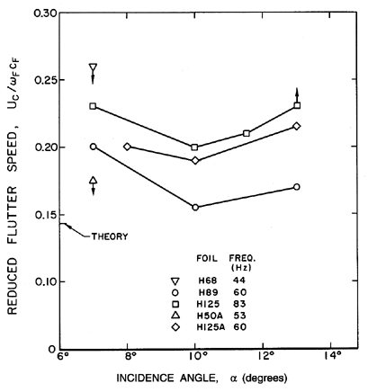
| Figure 8.22 Dimensionless critical flutter speeds for single supercavitating hydrofoils at various angles of incidence, α, and very long cavities (>5 chord lengths) (from Brennen, Oey, and Babcock 1980). |
The other major factor is the effect of cavitation. The changes which developed cavitation cause in the lift and drag characteristics of a single foil, also cause a fundamental change in the flutter characteristics with the result that a single cavitating foil can flutter (Abramson 1969). Thus a cavitating foil is unlike a noncavitating, nonseparated foil but qualitatively similar to a stalled foil whose flow it more closely resembles. Abramson (1969) provides a useful review of both the experiments and the analyses of flutter of rigid cavitating foils. However, as we previously remarked, the most likely form of flutter in a pump will not involve global blade motion but flexure of the leading or trailing edges. Since cavitation occurs at the leading edges, and since these are often made thin in order to optimize the hydraulic performance, leading edge flutter seems the most likely concern (figure 8.21). Data on this phenomenon was obtained by Brennen, Oey, and Babcock (1980), and is presented in figure 8.22. The critical incident fluid velocity, UC, is nondimensionalized using ωF, the lowest natural frequency of oscillation of the leading edge immersed in water, and a dimension, cF, that corresponds to the typical chordwise length of the foil from the leading edge to the first node of the first mode of vibration. The data shows that UC/cFωF is almost independent of the incidence angle, and is consistent for a wide range of natural frequencies. Brennen et al. also utilize the unsteady lift and moment coefficients calculated by Parkin (1962) to generate a theoretical estimate of UC/cFωF of 0.14. From figure 8.22 this seems to constitute an upper design limit on the reduced critical speed. Also note that the value of 0.14 is much smaller than the values of 1-3 quoted earlier for the stall flutter of a noncavitating foil. This difference emphasizes the enhanced flutter possibilities caused by cavitation. Brennen et al. also tested their foils under noncavitating conditions but found no sign of flutter even when the tunnel velocity was much larger than the cavitating flutter speed.
One footnote on the connection between the flutter characteristics of figure 8.22 and the partial cavitation oscillation of section 8.10 is worth adding. The data of figure 8.22 was obtained with long attached cavities, covering the entire suction surface of the foil as indicated in figure 8.21. At larger cavitation numbers, when the cavity length was decreased to about two chord lengths, the critical speed decreased markedly, and the leading edge flutter phenomenon began to metamorphose into the partial cavitation oscillation described in section 8.10.
8.13 POGO INSTABILITIES
All of the other discussion in this chapter has assumed that the turbomachine as a whole remains fixed in a nonaccelerating reference frame or, at least, that a vibrational degree of freedom of the machine is not necessary for the instability to occur. However, when a mechanism exists by which the internal flow and pressure oscillations can lead to vibration of the turbomachine as a whole, then a new set of possibilities are created. We refer to circumstances in which flow or pressure oscillations lead to vibration of the turbomachine (or its inlet or discharge pipelines) which in turn generate pressure oscillations that feed back to create instability. An example is the class of liquid-propelled rocket vehicle instabilities known as Pogo instabilities (NASA 1970). Here the longitudinal vibration of the rocket causes flow and pressure oscillation in the fuel tanks and, therefore, in the inlet lines. This, in turn, implies that the engines experience fluctuating inlet conditions, and as a result they produce a fluctuating thrust that promotes the longitudinal vibration of the vehicle. Rubin (1966) and Vaage et al. (1972) provide many of the details of these phenomena that are beyond the scope of this text. It is, however, important to note that the dynamics of the cavitating inducer pumps are crucial in determining the limits of these Pogo instabilities, and provide one of the main motivations for the measurements of the dynamic transfer functions of cavitating inducers described in chapter 9.
In closing, it is important to note that feedback systems involving vibrational motion of the turbomachine are certainly not confined to liquid propelled rockets. However, detailed examinations of the instabilities are mostly confined to this context. In section 9.15 of the next chapter, we provide a brief introduction to the frequency domain methods which can be used to address problems involving oscillatory, translational or rotational motions of the whole hydraulic system.
- Abramson, H.N. (1969). Hydroelasticity: a review of hydrofoil flutter. Appl. Mech. Rev., 22, No. 2, 115--121.
- Acosta, A.J. (1955). A note on partial cavitation of flat plate hydrofoils. Calif. Inst. of Tech. Hydro. Lab. Rep. E-19.9.
- Acosta, A.J. and DeLong, R.K. (1971). Experimental investigation of non-steady forces on hydrofoils oscillating in heave. Proc. IUTAM Symp. on non-steady flow of water at high speeds, Leningrad, USSR, 95--104.
- Adamczyk, J.J. (1975). The passage of a distorted velocity field through a cascade of airfoils. Proc. Conf. on Unsteady Phenomena in Turbomachinery, AGARD Conf. Proc. No. 177.
- Arndt, N., Acosta, A.J., Brennen, C.E., and Caughey, T.K. (1989). Rotor-stator interaction in a diffuser pump. ASME J. of Turbomachinery, 111, 213--221.
- Arndt, N., Acosta, A.J., Brennen, C.E., and Caughey, T.K. (1990). Experimental investigation of rotor-stator interaction in a centrifugal pump with several vaned diffusers. ASME J. of Turbomachinery, 112, 98--108.
- Badowski, H.R. (1969). An explanation for instability in cavitating inducers. ASME Cavitation Forum, 38--40.
- Braisted, D.M. and Brennen, C.E. (1980). Auto-oscillation of cavitating inducers. In Polyphase Flow and Transport Technology, (ed: R.A. Bajura), ASME Publ., New York, 157--166.
- Brennen, C.E., Oey, K., and Babcock, C.D. (1980). On the leading edge flutter of cavitating hydrofoils. J. Ship Res., 24, No. 3, 135--146.
- Brennen, C.E., Franz, R., and Arndt, N. (1988). Effects of cavitation on rotordynamic force matrices. Proc. Third Earth to Orbit Propulsion Conference, NASA Conf. Publ. 3012, 227--239.
- Chamieh, D.S., Acosta, A.J., Brennen, C.E., and Caughey, T.K. (1985). Experimental measurements of hydrodynamic radial forces and stiffness matrices for a centrifugal pump-impeller. ASME J. Fluids Eng., 107, No. 3, 307--315.
- Cumpsty, N. A. (1977). Review---a critical review of turbomachinery noise. ASME J. Fluids Eng., 99, 278--293.
- d'Agostino, L. and Brennen, C.E. (1983). On the acoustical dynamics of bubble clouds. ASME Cavitation and Multiphase Flow Forum, 72--75.
- Dean, R. C. (1959). On the necessity of unsteady flow in fluid machines. ASME J. Basic Eng., 81, 24--28.
- Dring, R.P., Joslyn, H.D., Hardin, L.W., and Wagner, J.H. (1982). Turbine rotor-stator interaction. ASME J. Eng. for Power, 104, 729--742.
- Dussourd, J. L. (1968). An investigation of pulsations in the boiler feed system of a central power station. ASME J. Basic Eng., 90, 607--619.
- Ek, B. (1957). Technische Strömungslehre. Springer-Verlag.
- Emmons, H.W., Pearson, C.E., and Grant, H.P. (1955). Compressor surge and stall propagation. Trans. ASME, 79, 455--469.
- Emmons, H.W., Kronauer, R.E., and Rockett, J.A. (1959). A survey of stall propagation---experiment and theory. ASME J. Basic Eng., 81, 409--416.
- Fung, Y.C. (1955). An introduction to the theory of aeroelasticity. John Wiley and Sons.
- Gallus, H.E. (1979). High speed blade-wake interactions. von Karman Inst. for Fluid Mech. Lecture Series 1979-3, 2.
- Gallus, H.E., Lambertz, J., and Wallmann, T. (1980). Blade-row interaction in an axial flow subsonic compressor stage. ASME J. Eng. for Power, 102, 169--177.
- Greitzer, E.M. (1976). Surge and rotating stall in axial flow compressors. Part I: Theoretical compression system model. Part II: Experimental results and comparison with theory. ASME J. Eng. for Power, 98, 190--211.
- Greitzer, E.M. (1981). The stability of pumping systems---the 1980 Freeman Scholar Lecture. ASME J. Fluids Eng., 103, 193--242.
- Ham, N.D. (1968). Aerodynamic loading on a two-dimensional airfoil during dynamic stall. AIAA J., 6, 1927--1934.
- Hartmann, M.J. and Soltis, R.F. (1960). Observation of cavitation in a low hub-tip ratio axial flow pump. Proc. Gas Turbine Power and Hydraulic Conf., ASME Paper No. 60-HYD-14.
- Hergt, P. and Benner, R. (1968). Visuelle Untersuchung der Strömung in Leitrad einer Radialpumpe. Schweiz. Banztg., 86, 716--720.
- Hobson, D. E. and Marshall, A. (1979). Surge in centrifugal pumps. Proc. 6th Conf. on Fluid Machinery, Budapest, 475--483.
- Horlock, J. M. (1968). Fluctuating lift forces on airfoils moving through transverse and chordwise gusts. ASME J. Basic Eng., 494--500.
- Iino, T. and Kasai, K. (1985). An analysis of unsteady flow induced by interaction between a centrifugal impeller and a vaned diffuser (in Japanese). Trans. Japan Soc. of Mech. Eng., 51, No.471, 154--159.
- Jaeger, C. (1963). The theory of resonance in hydro-power systems, discussion of incidents and accidents occurring in pressure systems. ASME J. Basic Eng., 85, 631--640.
- Jansen, W. 1964. Rotating stall in a radial vaneless diffuser. ASME J. Basic Eng., 86, 750--758.
- Kamijo, K., Shimura, T., and Watanabe, M. (1977). An experimental investigation of cavitating inducer instability. ASME Paper 77-WA/FW-14.
- Kamijo, K., Shimura, T., and Watanabe, M. (1980). A visual observation cavitating inducer instability. Nat. Aero. Lab. (Japan), Rept. NAL TR-598T.
- Kamijo, K., Yoshida, M., and Tsujimoto, Y. (1992). Hydraulic and mechanical performance of LE-7 LOX pump inducer. Proc. 28th Joint Propulsion Conf., Paper AIAA-92-3133.
- Kemp, N. H. and Ohashi, H. (1975). Forces on unstaggered airfoil cascades in unsteady in-phase motion with applications to harmonic oscillation. Proc. Symp. on Unsteady Aerodynamics, Tuscon, Ariz., 793--826.
- Kemp, N. H. and Sears, W. R. (1955). The unsteady forces due to viscous wakes in turbomachines. J. Aero Sci., 22, No.7, 478--483.
- Lefcort, M.D. (1965). An investigation into unsteady blade forces in turbomachines. ASME J. Eng. for Power, 87, 345--354.
- Leiblein, S. (1965). Experimental flow in two dimensional cascades. Chapter VI in Aerodynamic design of axial flow compressors, NASA SP-36.
- Lenneman, E. and Howard, J. H. G. (1970). Unsteady flow phenomena in centrifugal impeller passages. ASME J. Eng. for Power, 92-1, 65--72.
- Makay, E. and Szamody, O. (1978). Survey of feed pump outages. Electric Power Res. Inst. Rep. FP-754.
- Marscher, W.D. (1988). Subsynchronous vibration in boiler feed pumps due to stable response to hydraulic forces on at part-load. Proc. I.Mech.E. Conf. on Part Load Pumping, London, 167--175.
- Martin, M. (1962). Unsteady lift and moment on fully cavitating hydrofoils at zero cavitation number. J. Ship Res., 6, No.1, 15--25.
- McCroskey, W. J. (1977). Some current research in unsteady fluid dynamics---the 1976 Freeman Scholar Lecture. ASME J. Fluids Eng., 99, 8--38.
- Meyer, R.X. (1958). The effect of wakes on the transient pressure and velocity distributions in turbomachines. Trans. ASME, 80, 1544.
- Mikolajczak, A. A., Arnoldi, R. A., Snyder, L. E., and Stargardter, H. (1975). Advances in fan and compressor blade flutter analysis and predictions. J. Aircraft, 12, No.4, 325--332.
- Miller, C.D. and Gross, L.A. (1967). A performance investigation of an eight-inch hubless pump inducer in water and liquid nitrogen. NASA TN D-3807.
- Miskovish, R.S. and Brennen, C.E. (1992). Some unsteady fluid forces measured on pump impellers. ASME J. Fluids Eng., 114, 632--637.
- Miyagawa, K., Mutaguchi, K., Kanki, H., Iwasaki, Y., Sakamoto, A., Fujiki, S., Terasaki, A., and Furuya, S. (1992). An experimental investigation of fluid exciting force on a high head pump-turbine runner. Proc. 4th Int. Symp. on Transport Phenomena and Dynamics of Rotating Machinery, B, 133--142.
- Murai, H. (1968). Observations of cavitation and flow patterns in an axial flow pump at low flow rates (in Japanese). Mem. Inst. High Speed Mech., Tohoku Univ., 24, No.246, 315--333.
- NASA. (1970). Prevention of coupled structure-propulsion instability. NASA SP-8055.
- Natanzon, M.S., Bl'tsev, N.E., Bazhanov, V.V., and Leydervarger, M.R. (1974). Experimental investigation of cavitation-induced oscillations of helical inducers. Fluid Mech., Soviet Res., 3, No.1, 38--45.
- Parkin, B.R. (1962). Numerical data on hydrofoil reponse to non-steady motions at zero cavitation number. J. Ship Res., 6, 40--42.
- Platzer, M. F. (1978). Unsteady flows in turbomachines---a review of current developments. AGARD Rept. CP-227.
- Rosenmann, W. (1965). Experimental investigations of hydrodynamically induced shaft forces with a three bladed inducer. Proc. ASME Symp. on Cavitation in Fluid Machinery, 172--195.
- Rubin, S. (1966). Longitudinal instability of liquid rockets due to propulsion feedback (Pogo). J. Spacecraft and Rockets, 3, No.8, 1188--1195.
- Sack, L.E. and Nottage, H.B. (1965). System oscillations associated with cavitating inducers. ASME J. Basic Eng., 87, 917--924.
- Samoylovich, G.S. (1962). On the calculation of the unsteady flow around an array of arbitrary profiles vibrating with arbitrary phase shift. Prikladnaya Matematika i Mekhanika, No.4.
- Schorr, B. and Reddy, K.C. (1971). Inviscid flow through cascades in oscillatory and distorted flow. AIAA J., 9, 2043--2050.
- Silberman, E. and Song, C.S. (1961). Instability of ventilated cavities. J. Ship Res., 5, 13--33.
- Sisto, F. (1953). Stall-flutter in cascades. J. Aero. Sci., 20, 598--604.
- Sisto, F. (1967). Linearized theory of non-stationary cascades at fully stalled or supercavitating conditions. Zeitschrift fur Angewandte Mathematik und Mechanik, 8, 531--542.
- Sisto, F. (1977). A review of the fluid mechanics of aeroelasticity in turbomachines. ASME J. Fluids Eng., 99, 40--44.
- Song, C.S. (1962). Pulsation of ventilated cavities. J. Ship Res., 5, 8--20
- Sparks, C.R. and Wachel, J.C. (1976). Pulsations in liquid pumps and piping systems. Proc. 5th Turbomachinery Symp., 55--61.
- Strub, R.A. (1963). Pressure fluctuations and fatigue stresses in storage pumps and pump-turbines. ASME Paper No. 63-AHGT-11.
- Tsujimoto, Y., Imaichi, K., Tomohiro, T., and Gatoo, M. (1986). A two-dimensional analysis of unsteady torque on mixed flow impellers. ASME J. Fluids Eng., 108, No. 1, 26--33.
- Tsujimoto, Y., Kamijo, K., and Yoshida, Y. (1992). A theoretical analysis of rotating cavitation in inducers. ASME Cavitation and Multiphase Flow Forum, FED 135, 159--166.
- Tsukamoto, H. and Ohashi, H. (1982). Transient characteristics of centrifugal turbomachines. ASME J. Fluids Eng., 104, No. 1, 6--14.
- Tulin, M.P. (1953). Steady two-dimensional cavity flows about slender bodies. David Taylor Model Basin Rep. 834.
- Tyler, J.M. and Sofrin, T.G. (1962). Axial compressor noise studies. Soc. Automotive Eng., 70, 309--332.
- Vaage, R.D., Fidler, L.E., and Zehnle, R.A. (1972). Investigation of characteristics of feed system instabilities. Final Rept. MCR-72-107, Martin Marietta Corp., Denver, Col.
- van der Braembussche, R. (1982). Rotating stall in vaneless diffusers of centrifugal compressors. von Karman Inst. for Fluid Dyn., Technical Note 145.
- Verdon, J.M. (1985). Linearized unsteady aerodynamic theory. United Technologies Research Center Report R85-151774-1.
- Wade, R.B. and Acosta, A.J. (1966). Experimental observations on the flow past a plano-convex hydrofoil. ASME J. Basic Eng., 88, 273--283.
- Whitehead, D. (1960). Force and moment coefficients for vibrating airfoils in cascade. ARC R\&M 3254, London.
- Woods, L.C. (1955). On unsteady flow through a cascade of airfoils. Proc. Roy. Soc. A, 228, 50--65.
- Woods, L.C. (1957). Aerodynamic forces on an oscillating aerofoil fitted with a spoiler. Proc. Roy. Soc. A, 239, 328--337.
- Woods, L.C. (1961). The theory of subsonic plane flow. Cambridge Univ. Press.
- Yamamoto, K. (1991). Instability in a cavitating centrifugal pump. JSME Int. J., Ser. II, 34, 9--17.
- Yoshida, Y., Murakami, Y., Tsurusaki, T., and Tsujimoto, Y. (1991). Rotating stalls in centrifugal impeller/vaned diffuser systems. Proc. First ASME/JSME Joint Fluids Eng. Conf., FED-107, 125--130.
- Young, W.E., Murphy, R., and Reddecliff, J.M. (1972). Study of cavitating inducer instabilities. Pratt and Whitney Aircraft, Florida Research and Development Center, Rept. PWA FR-5131.
Last updated 12/1/00.
Christopher E. Brennen