HYDRODYNAMICS OF PUMPS
by Christopher Earls Brennen © Concepts NREC 1994
CHAPTER 6.
BUBBLE DYNAMICS, DAMAGE AND NOISE
6.1 INTRODUCTION
We now turn to the characteristics of cavitation for σ <σi. To place the material in context, we begin with a discussion of bubble dynamics, so that reference can be made to some of the classic results of that analysis. This leads into a discussion of two of the deleterious effects that occur as soon as there is any cavitation, namely cavitation damage and cavitation noise. In the next chapter, we address another deleterious consequence of cavitation, namely its effect upon hydraulic performance.
6.2 CAVITATION BUBBLE DYNAMICS
Two fundamental models for cavitation have been extensively used in the literature. One of these is the spherical bubble model which is most relevant to those forms of bubble cavitation in which nuclei grow to visible, macroscopic size when they encounter a region of low pressure, and collapse when they are convected into a region of higher pressure. For present purposes, we give only the briefest outline of these methods, while referring the reader to the extensive literature for more detail (see, for example, Knapp, Daily and Hammitt 1970, Plesset and Prosperetti 1977, Brennen 1994). The second fundamental methodology is that of free streamline theory, which is most pertinent to flows consisting of attached cavities or vapor-filled wakes; a brief review of this methodology is given in chapter 7.
Virtually all of the spherical bubble models are based on some version of the Rayleigh-Plesset equation (Plesset and Prosperetti 1977) that defines the relation between the radius of a spherical bubble, R(t), and the pressure, p(t), far from the bubble. In an otherwise quiescent incompressible Newtonian liquid, this equation takes the form
 | ......(6.1) |
 , and ρL are respectively the kinematic
viscosity, surface tension, and density of the liquid.
This equation (without the viscous and
surface tension terms) was first derived by Rayleigh (1917) and was
first applied to the problem of a traveling cavitation bubble by
Plesset (1949).
, and ρL are respectively the kinematic
viscosity, surface tension, and density of the liquid.
This equation (without the viscous and
surface tension terms) was first derived by Rayleigh (1917) and was
first applied to the problem of a traveling cavitation bubble by
Plesset (1949).
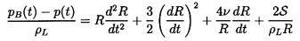
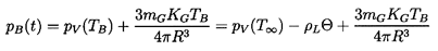
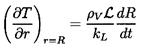
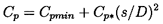
The pressure far from the bubble, p(t), is an input function that could be obtained from a determination of the pressure history that a nucleus would experience as it travels along a streamline. The pressure, pB(t), is the pressure inside the bubble. It is often assumed that the bubble contains both vapor and noncondensable gas, so that
 | ......(6.2) |
 | ......(6.3) |
 is the latent heat.
|
| Figure 6.1 Typical solution, R(t), of the Rayleigh-Plesset equation for a spherical bubble originating from a nucleus of radius, R0. The nucleus enters a low pressure region at a dimensionless time of 0 and is convected back to the original pressure at a dimensionless time of 500. The low pressure region is sinusoidal and symmetric about a dimensionless time of 250. |
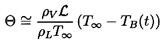
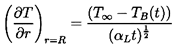
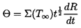
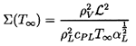
Note that in using equation 6.2 for pB(t), we have introduced the additional unknown function, TB(t), into the Rayleigh-Plesset equation 6.1. In order to determine this function, it is necessary to construct and solve a heat diffusion equation, and an equation for the balance of heat in the bubble. Approximate solutions to these equations can be written in the following simple form. If the heat conducted into the bubble is equated to the rate of use of latent heat at the interface, then
 | ......(6.4) |
 | ......(6.5) |
 | ......(6.6) |
 | ......(6.7) |
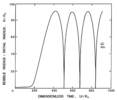
For present purposes, it is useful to illustrate some of the characteristic features of solutions to the Rayleigh-Plesset equation in the absence of thermal effects (Θ =0 and TB(t)=T∞). A typical solution of R(t) for a nucleus convected through a low pressure region is shown in figure 6.1. Note that the response of the bubble is quite nonlinear; the growth phase is entirely different in character from the collapse phase. The growth is steady and controlled; it rapidly reaches an asymptotic growth rate in which the dominant terms of the Rayleigh-Plesset equation are the pressure difference, pV-p, and the second term on the right-hand side so that
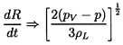 | ......(6.8) |
 | ......(6.9) |
|
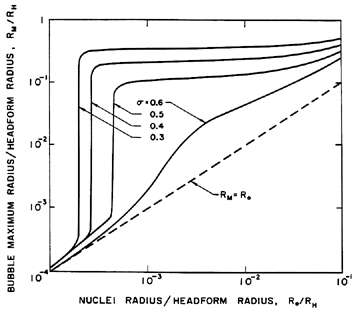
| Figure 6.2
The maximum size to which a cavitation bubble
grows (according to the Rayleigh-Plesset equation), RM, as function of
the original nuclei size, R0, and the cavitation number, σ,
in the flow around an axisymmetric headform of radius, RH,
with /ρL RH U2=0.000036 (from Ceccio and Brennen 1991).
|
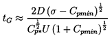
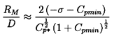
It follows that we can estimate the typical maximum size of a cavitation bubble, RM, given the above growth rate and the time available for growth. Numerical calculations using the full Rayleigh-Plesset equation show that the appropriate time for growth is the time for which the bubble experiences a pressure below the vapor pressure. In traveling bubble cavitation we may estimate this by knowing the shape of the pressure distribution near the minimum pressure point. We shall represent this shape by
 | ......(6.10) |
 | ......(6.11) |
 | ......(6.12) |
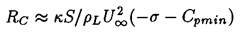
One other feature of the growth process is important to mention. It transpires that because of the stabilizing influence of the surface tension term, a particular tension, (pV-p), will cause only bubbles larger than a certain critical size to grow explosively (Blake 1949). This means that, for a given cavitation number, only nuclei larger than a certain critical size will achieve the growth rate necessary to become macroscopic cavitation bubbles. A decrease in the cavitation number will activate smaller nuclei, thus increasing the volume of cavitation. This phenomenon is illustrated in figure 6.2 which shows the maximum size of a cavitation bubble, RM, as a function of the size of the original nucleus and the cavitation number for a typical flow around an axisymmetric headform. The vertical parts of the curves on the left of the figure represent the values of the critical nuclei size, RC, that are, incidentally, given simply by the expression
 | ......(6.13) |
Turning now to the collapse, it is readily seen from figure 6.1 that cavitation bubble collapse is a catastrophic phenomenon in which the bubble, still assumed spherical, reaches a size very much smaller than the original nucleus. Very high accelerations and pressures are generated when the bubble becomes very small. However, if the bubble contains any noncondensable gas at all, this will cause a rebound as shown in figure 6.1. Theoretically, the spherical bubble will undergo many cycles of collapse and rebound. In practice, a collapsing bubble becomes unstable to nonspherical disturbances, and essentially shatters into many smaller bubbles in the first collapse and rebound. The resulting cloud of smaller bubbles rapidly disperses. Whatever the deviations from the spherical shape, the fact remains that the collapse is a violent process that produces noise and the potential for material damage to nearby surfaces. We proceed to examine both of these consequences in the two sections which follow.
|
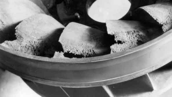
| Figure 6.3 Photograph of localized cavitation damage on the blade of a mixed flow pump impeller made from an aluminium-based alloy. |
|
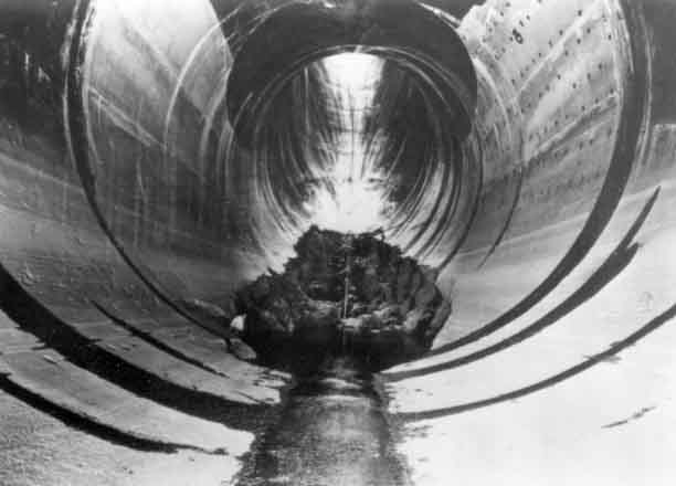
| Figure 6.4 Cavitation damage on the blades at the discharge from a Francis turbine. |
|
| Figure 6.5 Cavitation damage to the concrete wall of the 15.2m diameter Arizona spillway at the Hoover Dam. The hole is 35m long, 9m wide and 13.7m deep. Reproduced from Warnock (1945). |
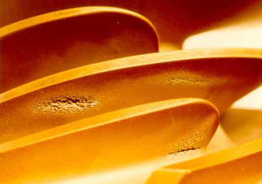
Perhaps the most ubiquitous problem caused by cavitation is the material damage that cavitation bubbles can cause when they collapse in the vicinity of a solid surface. Consequently, this aspect of cavitation has been intensively studied for many years (see, for example, ASTM 1967, Knapp, Daily, and Hammitt 1970, Thiruvengadam 1967, 1974). The problem is complex because it involves the details of a complicated unsteady flow combined with the reaction of the particular material of which the solid surface is made.
As we have seen in the previous section, cavitation bubble collapse is a violent process that generates highly localized, large amplitude disturbances and shocks in the fluid at the point of collapse. When this collapse occurs close to a solid surface, these intense disturbances generate highly localized and transient surface stresses. Repetition of this loading due a multitude of bubble collapses can cause local surface fatigue failure, and the detachment of pieces of material. This is the generally accepted explanation for cavitation damage. It is consistent with the appearance of cavitation damage in most circumstances. Unlike the erosion due to solid particles in the flow, for which the surface appears to be smoothly worn with scratches due to larger particles, cavitation damage has the crystalline and jagged appearance of fatigue failure. To illustrate this, a photograph of localized cavitation damage on the blade of a mixed flow pump, fabricated from an aluminium-based alloy, is included as 6.3. More extensive damage is illustrated in figure 6.4 which shows the blades at discharge from a Francis turbine; here the cavitation damage has penetrated the blades. Cavitation damage can also occur in much larger scale flows. As an example, figure 6.5 shows cavitation damage suffered by a spillway at the Hoover dam (Warnock 1945, Falvey 1990).
|
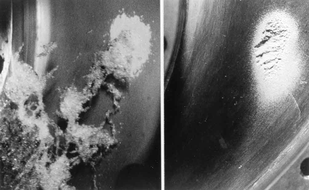
| Figure 6.6 Axial views from the inlet of the cavitation and cavitation damage on the hub or base plate of a centrifugal pump impeller. The two photographs are of the same area, the left one showing the typical cavitation pattern during flow and the right one the typical cavitation damage. Parts of the blades can be seen in the upper left and lower right corners; relative to these blades the flow proceeds from the lower left to the upper right. The leading edge of the blade is just outside the field of view on the upper left. Reproduced from Soyama, Kato and Oba (1992) with permission of the authors. |
In hydraulic devices such as pump impellers or propellers, cavitation damage is often observed to occur in quite localized areas of the surface. This is frequently the result of the periodic and coherent collapse of a cloud of cavitation bubbles. Such is the case in magnetostrictive cavitation testing equipment (Knapp, Daily, and Hammitt 1970). In many pumps, the periodicity may occur naturally as a result of regular shedding of cavitating vortices, or it may be a response to a periodic disturbance imposed on the flow. Examples of the kinds of imposed fluctuations are the interaction between a row of rotor vanes and a row of stator vanes, or the interaction between a ship's propeller and the nonuniform wake behind the ship. In almost all such cases, the coherent collapse of the cloud can cause much more intense noise and more potential for damage than in a similar nonfluctuating flow. Consequently, the damage is most severe on the solid surface close to the location of cloud collapse. An example of this phenomenon is included in figure 6.6 taken from Soyama, Kato and Oba (1992). In this instance, clouds of cavitation are being shed from the leading edge of a centrifugal pump blade, and are collapsing in a specific location as suggested by the pattern of cavitation in the left-hand photograph. This leads to the localized damage shown in the right-hand photograph.
Currently, several research efforts are focussed on the dynamics of cavitation clouds. These studies suggest that the coherent collapse can be more violent than that of individual bubbles, but the basic explanation for the increase in the noise and damage potential is not clear.
6.4 MECHANISM OF CAVITATION DAMAGE
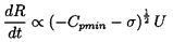
The intense disturbances that are caused by cavitation bubble collapse can have two separate origins. The first is related to the fact that a collapsing bubble may be unstable in terms of its shape. When the collapse occurs near a solid surface, Naude and Ellis (1961) and Benjamin and Ellis (1966) observed that the developing spherical asymmetry takes the form of a rapidly accelerating jet of fluid, entering the bubble from the side furthest from the wall (see figure 6.7). Plesset and Chapman (1971) carried out numerical calculations of this ``reentrant jet'', and found good agreement with the experimental observations of Lauterborn and Bolle (1975). Since then, other analytical methods have explored the parametric variations in the flow. These methods are reviewed by Blake and Gibson (1987). The ``microjet'' achieves very high speeds, so that its impact on the other side of the bubble generates a shock wave, and a highly localized shock loading of the surface of the nearby wall.
|
| Figure 6.7 The collapse of a cavitation bubble close to a solid boundary. The theoretical shapes of Plesset and Chapman (1971) (solid lines) are compared with the experimental observations of Lauterborn and Bolle (1975) (points) (adapted from Plesset and Prosperetti 1977). |
Parenthetically, we might remark that this is also the principle on which the depth charge works. The initial explosion creates little damage, but does produce a very large bubble which, when it collapses, generates a reentrant jet directed toward any nearby solid surface. When this surface is a submarine, the collapse of the bubble can cause great damage to that vessel. It may also be of interest to note that a bubble, collapsing close to a very flexible or free surface, develops a jet on the side closest to this boundary, and, therefore, traveling in the opposite direction. Some researchers have explored the possibility of minimizing cavitation damage by using surface coatings with a flexibility designed to minimize the microjet formation.
The second intense disturbance occurs when the remnant cloud of bubbles, that remains after the microjet disruption, collapses to its minimum gas/vapor volume, and generates a second shock wave that impinges on the nearby solid surface. The generation of a shock wave during the rebound phase of bubble motion was first demonstrated by the calculations of Hickling and Plesset (1964). More recently, Shima et al. (1981) have made interesting observations of the spherical shock wave using Schlieren photography, and Fujikawa and Akamatsu (1980) have used photoelastic solids to examine the stress waves developed in the solid. Though they only observed stress waves resulting from the remnant cloud collapse and not from the microjet, Kimoto (1987) has subsequently shown that both the microjet and the remnant cloud create stress waves in the solid. His measurements indicate that the surface loading resulting from the remnant cloud is about two or three times that due to the microjet.
Until very recently, virtually all of these detailed observations of collapsing cavitation bubbles had been made in a quiescent fluid. However, several recent observations have raised doubts regarding the relevance of these results for most flowing systems. Ceccio and Brennen (1991) have made detailed observations of the collapse of cavitating bubbles in flows around bodies, and have observed that typical cavitation bubbles are distorted and often broken up by the shear in the boundary layer or by the turbulence before the collapse takes place. Furthermore, Chahine (personal communication) has performed calculations similar to those of Plesset and Chapman, but with the addition of rotation due to shear, and has found that the microjet is substantially modified and reduced by the flow.
|
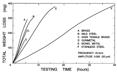
| Figure 6.8 Examples of cavitation damage weight loss as a function of time. Data from vibratory tests with different materials (Hobbs, Laird and Brunton 1967). |
|
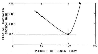
| Figure 6.9 Cavitation erosion rates in a centrifugal pump as a function of the flow rate relative to the design flow rate (Pearsall 1978 from Grist 1974). |
The other important facet of the cavitation damage phenomenon is the reaction of the material of the solid boundary to the repetitive shock (or ``water hammer'') loading. Various measures of the resistance of particular materials to cavitation damage have been proposed (see, for example, Thiruvengadam 1967). These are largely heuristic and empirical, and will not be reviewed here. The reader is referred to Knapp, Daily, and Hammitt (1970) for a detailed account of the relative resistance of different materials to cavitation damage. Most of these comparisons are based, not on tests in flowing systems, but on results obtained when material samples are vibrated at high frequency (about 20kHz) in a bath of quiescent liquid. The samples are weighed at regular intervals to determine the loss of material, and the results are presented in the form typified by figure 6.8. Note that the relative erosion rates, according to this data, can be approximately correlated with the structural strength of the material. Furthermore, the erosion rate is not necessarily constant with time. This may be due to the differences in the response of a collapsing bubble to a smooth surface as opposed to a surface already roughened by damage. Finally, note that the weight loss in many materials only begins after a certain incubation time.
The data on erosion rates in pumps is very limited because of the length of time necessary to make such measurements. The data that does exist (Mansell 1974) demonstrates that the rate of erosion is a strong function of the operating point as given by the cavitation number and the flow coefficient. The influence of the latter is illustrated in figure 6.9. This curve essentially mirrors those of figures 5.16 and 5.17. At off-design conditions, the increased angle of incidence leads to increased cavitation and, therefore, increased weight loss.
6.5 CAVITATION NOISE
|
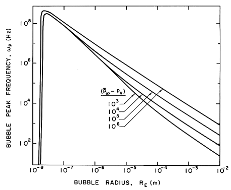
| Figure 6.10 Bubble natural frequency, ωP, in Hz as a function of the bubble radius and the difference between the equilibrium pressure and the vapor pressure (in kg/m sec2) for water at 300°K. |
|
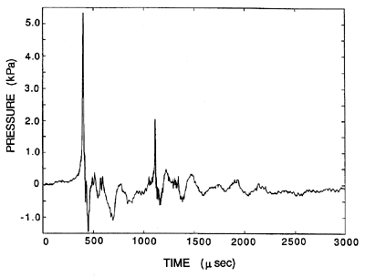
| Figure 6.11 Typical acoustic signal from a single collapsing bubble (from Ceccio and Brennen 1991). |
The violence of cavitation bubble collapse also produces noise. In many practical circumstances, the noise is important not only because of the vibration that it may cause, but also because it advertizes the presence of cavitation and, therefore, the likelihood of cavitation damage. Indeed, the magnitude of cavitation noise is often used as a crude measure of the rate of cavitation erosion. For example, Lush and Angell (1984) have shown that, in a given flow at a given cavitation number, the rate of weight loss due to cavitation damage is correlates with the noise as the velocity of the flow is changed.
Prior to any discussion of cavitation noise, it is useful to identify the
natural frequency with which individual
bubbles will oscillate a quiescent liquid.
This natural frequency can be obtained from the
Rayleigh-Plesset equation 6.1 by substituting an expression for R(t)
that consists of a constant, RE, plus a small sinusoidal
perturbation of amplitude,
 ,
at a general frequency, ω. Steady state
oscillations like this would only be maintained by an applied pressure,
p(t), consisting of a constant,
,
at a general frequency, ω. Steady state
oscillations like this would only be maintained by an applied pressure,
p(t), consisting of a constant,
 ,
plus a sinusoidal perturbation
of amplitude,
,
plus a sinusoidal perturbation
of amplitude,
 ,
and frequency, ω. Obtaining the relation
between the linear perturbations,
and
,
from the Rayleigh-Plesset equation, it is found that the ratio,
/,
has a maximum at a resonant frequency,
ωP, given by
,
and frequency, ω. Obtaining the relation
between the linear perturbations,
and
,
from the Rayleigh-Plesset equation, it is found that the ratio,
/,
has a maximum at a resonant frequency,
ωP, given by
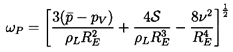 | ......(6.14) |
.
Note that the bubbles below about 0.02μm are supercritically damped,
and have no resonant frequency. Typical cavitation nuclei of size
10→ 100μm have resonant frequencies in the range
10→ 100kHz. Even though the nuclei are excited in a highly
nonlinear way by the cavitation, one might expect that the
spectrum of the noise that this process produces would have
a broad maximum at
the peak frequency corresponding to the size of the most numerous nuclei
participating in the cavitation. Typically, this would correspond to the
radius of the critical nucleus given by the expression 6.13.
For example, if the critical nuclei size were of the order of
10-100μm, then, according to figure 6.10, one might expect to
see cavitation noise frequencies of the order of 10-100kHz.
This is, indeed, the typical range of frequencies produced by cavitation.

|
| Figure 6.12 The acoustic impulse, I, produced by the collapse of a single cavitation bubble. Data is shown for two axisymmetric bodies (the ITTC and Schiebe headforms) as a function of the maximum volume prior to collapse. Also shown are the equivalent results from solutions of the Rayleigh-Plesset equation (from Ceccio and Brennen 1991). |
|
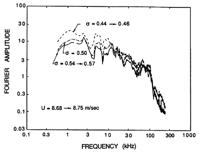
| Figure 6.13 Typical spectra of noise from bubble cavitation for various cavitation numbers as indicated (Ceccio and Brennen 1991). |
|
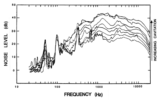
| Figure 6.14 Typical spectra showing the increase in noise with increasing cavitation in an axial flow pump (Lee 1966). |
Fitzpatrick and Strasberg (1956) were the first to make extensive use of the Rayleigh-Plesset equation to predict the noise from individual collapsing bubbles and the spectra that such a process would produce. More recently, Ceccio and Brennen (1991) have recorded the noise from individual cavitation bubbles in a flow. A typical acoustic signal is reproduced in 6.11. The large positive pulse at about 450μs corresponds to the first collapse of the bubble. Since the radiated acoustic pressure, pA, in this context is related to the second derivative of the volume of the bubble, V(t), by
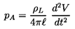 | ......(6.15) |
A good measure of the magnitude of the collapse pulse in figure 6.11 is the acoustic impulse, I, defined as the area under the curve or
 | ......(6.16) |
|
| Figure 6.15 The relation between the cavitation performance, the noise and vibration produced at three frequency levels in a centrifugal pump, namely the shaft frequency (squares), the blade passage frequency (upsidedown triangles) and 40kHz (circles) (Pearsall 1966-67). |
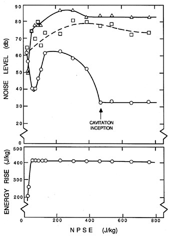
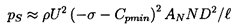
The typical single bubble noise shown in figure 6.11 leads to the spectrum shown in figure 6.13. If the cavitation events are randomly distributed in time, this would also correspond to the overall cavitation noise spectrum. It displays a characteristic frequency content in the range of 1→ 50kHz (the rapid decline at about 80kHz represents the limit of the hydrophone used to make these measurements). Typical measurements of the noise produced by cavitation in an axial flow pump are illustrated in figure 6.14, and exhibit the same features demonstrated in figure 6.13. The signal in figure 6.14 also clearly contains some shaft or blade passage frequencies that occur in the absence of cavitation, but may be amplified or attenuated by cavitation. Figure 6.15 contains data obtained for cavitation noise in a centrifugal pump. Note that the noise at a frequency of 40kHz shows a sharp increase with the onset of cavitation; on the other hand, the noise at the shaft and blade passage frequencies show only minor changes with cavitation number. The decrease in the 40kHz cavitation noise as breakdown is approached is also a common feature in cavitation noise measurements.
The level of the sound produced by a cavitating flow is the result of two
factors, namely the impulse, I, produced by each event (equation
6.16) and the event rate or number of
events per second,
 .
Therefore, the sound pressure
level, pS, will be
.
Therefore, the sound pressure
level, pS, will be
 | ......(6.17) |
,
and thus the scaling of the
cavitation noise, pS. We
emphasize that the following equations omit some factors of proportionality
necessary for quantitative calculations.
Both the experimental observations and the calculations based on the Rayleigh-Plesset equation, show that the nondimensional impulse from a single cavitation event, defined by
 | ......(6.18) |
 | ......(6.19) |
 | ......(6.20) |
Modeling the event rate,
, can be considerably more
complicated than might, at first sight, be visualized. If all the nuclei
flowing through a certain
known streamtube (say with a cross-sectional area, AN, in the upstream
reference flow), were to cavitate similarly then, clearly, the
result would be
 | ......(6.21) |
 | ......(6.22) |
Different scaling laws will apply when the cavitation is generated by turbulent fluctuations, such as in a turbulent jet (see, for example, Ooi 1985, Franklin and McMillan 1984). Then the typical tension and the typical duration of the tension experienced by a nucleus, as it moves along an approximately Lagrangian path in the turbulent flow, are very much more difficult to estimate. Consequently, estimates of the sound pressure due to cavitation in turbulent flows, and the scaling of that sound with velocity, are more poorly understood.
- ASTM (Amer. Soc. for Testing and Materials). (1967). Erosion by cavitation or impingement. ASTM STP408.
- Arakeri, V.H. and Shangumanathan, V. (1985). On the evidence for the effect of bubble interference on cavitation noise. J. Fluid Mech., 159, 131--150.
- Benjamin, T.B. and Ellis, A.T. (1966). The collapse of cavitation bubbles and the pressures thereby produced against solid boundaries. Phil. Trans. Roy. Soc., London, Ser. A, 260, 221--240.
- Blake, F.G. (1949). The onset of cavitation in liquids: I. Acoustics Res. Lab., Harvard Univ., Tech. Memo. No. 12.
- Blake, W.K., Wolpert, M.J., and Geib, F.E. (1977). Cavitation noise and inception as influenced by boundary-layer development on a hydrofoil. J. Fluid Mech., 80, 617--640.
- Blake, J.R. and Gibson, D.C. (1987). Cavitation bubbles near boundaries. Ann. Rev. Fluid Mech., 19, 99--124.
- Brennen, C.E. (1994). Cavitation and bubble dynamics. Oxford Univ. Press.
- Ceccio, S.L. and Brennen, C.E. (1991). Observations of the dynamics and acoustics of travelling bubble cavitation. J. Fluid Mech., 233, 633--660. Corrigenda, 240, 686.
- Falvey, H.T. (1990). Cavitation in chutes and spillways. US Bur. of Reclamation, Eng. Monograph No. 42.
- Fitzpatrick, H.M. and Strasberg, M. (1956). Hydrodynamic sources of sound. Proc. First ONR Symp. on Naval Hydrodynamics, 241--280.
- Franklin, R.E. and McMillan, J. (1984). Noise generation in cavitating flows, the submerged jet. ASME J. Fluids Eng., 106, 336--341.
- Fujikawa, S. and Akamatsu, T. (1980). Effects of the non-equilibrium condensation of vapour on the pressure wave produced by the collapse of a bubble in a liquid. J. Fluid Mech., 97, 481--512.
- Grist, E. (1974). NPSH requirements for avoidance of unacceptable cavitation erosion in centrifugal pumps. Proc. I.Mech.E. Conf. on Cavitation, 153--163.
- Hickling, R. and Plesset, M.S. (1964). Collapse and rebound of a spherical bubble in water. Phys. Fluids, 7, 7--14.
- Hobbs, J.M., Laird, A., and Brunton, W.C. (1967). Laboratory evaluation of the vibratory cavitation erosion test. Nat. Eng. Lab. (U.K.), Report No. 271.
- Kimoto, H. (1987). An experimental evaluation of the effects of a water microjet and a shock wave by a local pressure sensor. ASME Int. Symp. on Cavitation Res. Fac. and Techniques, FED 57, 217--224.
- Knapp, R.T., Daily, J.W., and Hammitt, F.G. (1970). Cavitation. McGraw-Hill, New York.
- Lauterborn, W. and Bolle, H. (1975). Experimental investigations of cavitation bubble collapse in the neighborhood of a solid boundary. J. Fluid Mech., 72, 391--399.
- Lee, C.J.M. (1966). Written discussion in Proc. Symp. on Pump Design, Testing and Operation, Natl. Eng. Lab., Scotland, 114-115.
- Lush, P.A. and Angell, B. (1984). Correlation of cavitation erosion and sound pressure level. ASME J. Fluids Eng., 106, 347--351.
- Mansell, C.J. (1974). Impeller cavitation damage on a pump operating below its rated discharge. Proc. of Conf. on Cavitation, Inst. of Mech. Eng., 185--191.
- Naude, C.F. and Ellis, A.T. (1961). On the mechanism of cavitation damage by non-hemispherical cavities in contact with a solid boundary. ASME. J. Basic Eng., 83, 648--656.
- Ooi, K.K. (1985). Scale effects on cavitation inception in submerged water jets: a new look. J. Fluid Mech., 151, 367--390.
- Pearsall, I.S. (1966-67). Acoustic detection of cavitation. Proc. Inst. Mech. Eng., 181, No. 3A.
- Pearsall, I.S. (1978). Off-design performance of pumps. von Karman Inst. for Fluid Dynamics, Lecture Series 1978-3.
- Plesset, M.S. (1949). The dynamics of cavitation bubbles. ASME J. Appl. Mech., 16, 228--231.
- Plesset, M.S. and Chapman, R.B. (1971). Collapse of an initially spherical vapor cavity in the neighborhood of a solid boundary. J. Fluid Mech., 47, 283--290.
- Plesset, M.S. and Prosperetti, A. (1977). Bubble dynamics and cavitation. Ann. Rev. Fluid Mech., 9, 145--185.
- Rayleigh, Lord. (1917). On the pressure developed in a liquid during the collapse of a spherical cavity. Phil. Mag., 34, 94--98.
- Shima, A., Takayama, K., Tomita, Y., and Muira, N. (1981). An experimental study on effects of a solid wall on the motion of bubbles and shock waves in bubble collapse. Acustica, 48, 293--301.
- Soyama, H., Kato, H., and Oba, R. (1992). Cavitation observations of severely erosive vortex cavitation arising in a centrifugal pump. Proc. Third I.Mech.E. Int. Conf. on Cavitation, 103--110.
- Thiruvengadam, A. (1967). The concept of erosion strength. Erosion by cavitation or impingement. ASTM STP 408, Am. Soc. Testing Mats., 22.
- Thiruvengadam, A. (1974). Handbook of cavitation erosion. Tech. Rep. 7301-1, Hydronautics, Inc., Laurel, Md.
- Warnock, J.E. (1945). Experiences of the Bureau of Reclamation. Proc. Amer. Soc. Civil Eng., 71, No.7, 1041--1056.
Last updated 12/1/00.
Christopher E. Brennen