HYDRODYNAMICS OF PUMPS
by Christopher Earls Brennen © Concepts NREC 1994
CHAPTER 5.
CAVITATION PARAMETERS AND INCEPTION
5.1 INTRODUCTION
This chapter will deal with the parameters that are used to describe cavitation, and the circumstances that govern its inception. In subsequent chapters, we address the deleterious effects of cavitation, namely cavitation damage, noise, the effect of cavitation on hydraulic performance, and cavitation-induced instabilities.
Cavitation is the process of the formation of vapor bubbles in low pressure regions within a flow. One might imagine that vapor bubbles are formed when the pressure in the liquid reaches the vapor pressure, pV, of the liquid at the operating temperature. While many complicating factors discussed later cause deviations from this hypothesis, nevertheless it is useful to adopt this as a criterion for the purpose of our initial discussion. In practice, it can also provide a crude initial guideline.
The static pressure, p, in any flow is normally nondimensionalized as a pressure coefficient, Cp, defined as
 | ......(5.1) |
 | ......(5.2) |
 | ......(5.3) |
Traditionally, several special dimensionless parameters are utilized in evaluating the potential for cavitation. Perhaps the most fundamental of these is the cavitation number, σ, defined as
 | ......(5.4) |
 | ......(5.5) |
Several variations in the definition of cavitation number occur in the literature. Often the inlet tip velocity, Ω RT1, is employed as the reference velocity, U, and this version will be used in this monograph unless otherwise stated. Sometimes, however, the relative velocity at the inlet tip, wT1, is used as the reference velocity, U. Usually the magnitudes of wT1 and Ω RT1 do not differ greatly, and so the differences in the two cavitation numbers are small.
In the context of pumps and turbines, a number of other, surrogate cavitation parameters are frequently used in addition to some special terminology. The NPSP (for net positive suction pressure) is an acronym used for (pT1-pV), where pT1 is the inlet total pressure given by
 | ......(5.6) |
 | ......(5.7) |
 | ......(5.8) |
The suction specific speed is similar in concept to the cavitation number in that it represents a nondimensional version of the inlet or suction pressure. Moreover, there will be a certain critical value of the suction specific speed at which cavitation first appears. This special value is termed the inception suction specific speed, Si. The reader should note that frequently, when a value of the ``suction specific speed'' is quoted for a pump, the value being given is some critical value of S that may or may not correspond to Si. More frequently, it corresponds to Sa, the value at which the degradation in the head rise reaches a certain percentage value (see section 5.5).
The suction specific speed, S, may be obtained from the cavitation number, σ, and vice versa, by noting that, from the relations 2.17, 5.4, 5.6, and 5.8, it follows that
 | ......(5.9) |
 | ......(5.10) |
 | ......(5.11) |
For illustrative purposes in the last section, we employed the criterion that cavitation occurs when the minimum pressure in the flow just reaches the vapor pressure, σi=-Cpmin. If this were the case, the prediction of cavitation would be a straightforward matter. Unfortunately, large departures from this criterion can occur in practice, and, in this section, we shall try to present a brief overview of the reasons for these discrepancies. There is, of course, an extensive body of literature on this subject, and we shall not attempt a comprehensive review. The reader is referred to reviews by Knapp, Daily and Hammit (1970), Acosta and Parkin (1975), Arakeri (1979) and Brennen (1994) for more detail.
|
| Figure 5.1 The inception numbers measured for the same axisymmetric headform in a variety of water tunnels around the world. Data collected as part of a comparative study of cavitation inception by the International Towing Tank Conference (Lindgren and Johnsson 1966, Johnsson 1969). |
First, it is important to recognize that vapor does not necessarily form when the pressure, p, in a liquid falls below the vapor pressure, pV. Indeed, a pure liquid can, theoretically, sustain a tension, Δ p=pV-p, of many atmospheres before nucleation, or the appearance of vapor bubbles, occurs. Such a process is termed homogeneous nucleation, and has been observed in the laboratory with some pure liquids (not water) under very clean conditions. In real engineering flows, these large tensions do not occur because vapor bubbles grow from nucleation sites either on the containing surfaces or suspended in the liquid. As in the case of a solid, the ultimate strength is determined by the weaknesses (stress concentrations) represented by the nucleation sites or ``nuclei.'' Research has shown that suspended nuclei are more important than surface nucleation sites in determining cavitation inception. These suspended nuclei may take the form either of microbubbles or of solid particles within which, perhaps, there are microbubbles. For example, a microbubble of radius, RN, containing only vapor, is in equilibrium when the liquid pressure
 | ......(5.12) |
 is the surface tension. It follows that such a
microbubble would result in a critical tension of
2/RN, and the liquid pressure would have to
fall below pV-2/RN before the
microbubble would grow to
a visible size. For example, a 10μm bubble in water at normal
temperatures leads to a tension of 0.14 bar.
is the surface tension. It follows that such a
microbubble would result in a critical tension of
2/RN, and the liquid pressure would have to
fall below pV-2/RN before the
microbubble would grow to
a visible size. For example, a 10μm bubble in water at normal
temperatures leads to a tension of 0.14 bar.
It is virtually impossible to remove all the particles, microbubbles and dissolved air from any substantial body of liquid (the catch-all term ``liquid quality'' is used to refer to the degree of contamination). Because of this contamination, substantial differences in the inception cavitation number (and, indeed, the form of cavitation) have been observed in experiments in different water tunnels, and even in a single facility with differently processed water. The ITTC comparative tests (Lindgren and Johnsson 1966, Johnsson 1969) provided a particularly dramatic example of these differences when cavitation on the same axisymmetric headform was examined in many different water tunnels around the world. An example of the variation of σi in those experiments, is reproduced as 5.1.
|
| Figure 5.2 Several nuclei number distribution functions measured in water tunnels and in the ocean by various methods (adapted from Gates and Acosta 1978). |
Because the cavitation nuclei are crucial to an understanding of cavitation inception, it is now recognized that the liquid in any cavitation inception study must be monitored by measuring the number of nuclei present in the liquid. This information is normally presented in the form of a nuclei number distribution function, N(RN), defined such that the number of nuclei per unit total volume with radii between RN and RN+dRN is given by N(RN)dRN. Typical nuclei number distributions are shown in figure 5.2 where data from water tunnels and from the ocean are presented.
Most of the methods currently used for making these measurements are still in the development stage. Devices based on acoustic scattering, and on light scattering, have been explored. Other instruments, known as cavitation susceptibility meters, cause samples of the liquid to cavitate, and measure the number and size of the resulting macroscopic bubbles. Perhaps the most reliable method has been the use of holography to create a magnified three-dimensional photographic image of a sample volume of liquid that can then be surveyed for nuclei. Billet (1985) has recently reviewed the current state of cavitation nuclei measurements (see also Katz et al 1984).
It may be interesting to note that cavitation itself is a source of nuclei in many facilities. This is because air dissolved in the liquid will tend to come out of solution at low pressures, and contribute a partial pressure of air to the contents of any macroscopic cavitation bubble. When that bubble is convected into a region of higher pressure and the vapor condenses, this leaves a small air bubble that only redissolves very slowly, if at all. This unforeseen phenomenon caused great difficulty for the first water tunnels which were modeled directly on wind tunnels. It was discovered that, after a few minutes of operating with a cavitating body in the working section, the bubbles produced by the cavitation grew rapidly in number, and began to complete the circuit of the facility so that they appeared in the incoming flow. Soon the working section was obscured by a two-phase flow. The solution had two components. First, a water tunnel needs to be fitted with a long and deep return leg so that the water remains at high pressure for sufficient time to redissolve most of the cavitation-produced nuclei. Such a return leg is termed a ``resorber''. Second, most water tunnel facilities have a ``deaerator'' for reducing the air content of the water to 20-50% of the saturation level at atmospheric pressure. These comments serve to illustrate the fact that N(RN) in any facility can change according to the operating condition, and can be altered both by deaeration and by filtration.
Most of the data of figure 5.2 is taken from water tunnel water that has been somewhat filtered and degassed, or from the ocean which is surprisingly clean. Thus, there are few nuclei with a size greater than 100μm. On the other hand, it is quite possible in many pump applications to have a much larger number of larger bubbles and, in extreme situations, to have to contend with a two-phase flow. Gas bubbles in the inflow could grow substantially as they pass through the low pressure regions within the pump, even though the pressure is everywhere above the vapor pressure. Such a phenomenon is called pseudo-cavitation. Though a cavitation inception number is not particularly relevant to such circumstances, attempts to measure σi under these circumstances would clearly yield values larger than -Cpmin.
On the other hand, if the liquid is quite clean with only very small nuclei, the tension that this liquid can sustain means that the minimum pressure has to fall well below pV for inception to occur. Then σi is much smaller than -Cpmin. Thus the quality of the water and its nuclei can cause the cavitation inception number to be either larger or smaller than -Cpmin.
There are, however, at least two other factors that can affect σi, namely the residence time and turbulence. The residence time effect arises because the nuclei must remain at a pressure below the critical value for a sufficient length of time to grow to observable size. This requirement will depend on both the size of the pump and the speed of the flow. It will also depend on the temperature of the liquid for, as we shall see later, the rate of bubble growth may depend on the temperature of the liquid. The residence time effect requires that a finite region of the flow be below the critical pressure, and, therefore, causes σi to be lower than might otherwise be expected.
Up to this point we have assumed that the flow and the pressures are laminar and steady. However, most of the flows with which one must deal in turbomachinery are not only turbulent but also unsteady. Vortices occur because they are inherent in turbulence and because of both free and forced shedding of vortices. This has important consequences for cavitation inception, because the pressure in the center of a vortex may be significantly lower than the mean pressure in the flow. The measurement or calculation of -Cpmin would elicit the value of the lowest mean pressure, while cavitation might first occur in a transient vortex whose central pressure was lower than the lowest mean pressure. Unlike the residence time factor, this would cause higher values of σi than would otherwise be expected. It would also cause σi to change with Reynolds number, Re. Note that this would be separate from the effect of Reynolds number on the minimum pressure coefficient, Cpmin. Note also that surface roughness can promote cavitation by creating localized low pressure perturbations in the same manner as turbulence.
5.4 SCALING OF CAVITATION INCEPTION
The complexity of the issues raised in the last section helps to explain why serious questions remain as to how to scale cavitation inception. This is perhaps one of the most troublesome issues that the developer of a liquid turbomachine must face. Model tests of a ship's propeller or large turbine (to quote two common examples) may allow the designer to accurately estimate the noncavitating performance of the device. However, he will not be able to place anything like the same confidence in his ability to scale the cavitation inception data.
Consider the problem in more detail. Changing the size of the device will alter not only the residence time effect but also the Reynolds number. Furthermore, the nuclei will now be a different size relative to the impeller. Changing the speed in an attempt to maintain Reynolds number scaling may only confuse the issue by also altering the residence time. Moreover, changing the speed will also change the cavitation number, and, to recover the modeled condition, one must then change the inlet pressure which may alter the nuclei content. There is also the issue of what to do about the surface roughness in the model and in the prototype.
The other issue of scaling that arises is how to anticipate the cavitation phenomena in one liquid based on data in another. It is clearly the case that the literature contains a great deal of data on water as the fluid. Data on other liquids is quite meager. Indeed the author has not located any nuclei number distributions for a fluid other than water. Since the nuclei play such a key role, it is not surprising that our current ability to scale from one liquid to another is quite tentative.
It would not be appropriate to leave this subject without emphasizing that most of the remarks in the last two sections have focused on the inception of cavitation. Once cavitation has become established, the phenomena that occur are much less sensitive to special factors, such as the nuclei content. Hence the scaling of developed cavitation can be anticipated with much more confidence than the scaling of cavitation inception. This is not, however, of much solace to the engineer charged with avoiding cavitation completely.
5.5 PUMP PERFORMANCE
|
| Figure 5.3 Schematic of noncavitating performance, ψ(φ), and cavitating performance, ψ(φ,σ), showing the three key cavitation numbers. |
The performance of a pump when presented nondimensionally will take the generic form sketched in figure 5.3. As discussed earlier, the noncavitating performance will consist of the head coefficient, ψ, as a function of the flow coefficient, φ, where the design conditions can be identified as a particular point on the ψ(φ) curve. The noncavitating characteristic should be independent of the speed, Ω, though at lower speeds there may be some deviation due to viscous or Reynolds number effects. The cavitating performance, as illustrated on the right in figure 5.3, is presented as a family of curves, ψ(φ,σ), each for a specific flow coefficient, in a graph of the head coefficient against cavitation number, σ. Frequently, of course, both performance curves are presented dimensionally; then, for example, the NPSH is often used instead of the cavitation number as the abscissa for the cavitation performance graph.
It is valuable to identify three special cavitation numbers in the cavitation performance graph. Consider a pump operating at a particular flow rate or flow coefficient, while the inlet pressure, NPSH, or cavitation number is gradually reduced. As discussed in the previous chapter, the first critical cavitation number to be reached is that at which cavitation first appears; this is called the cavitation inception number, σi. Often the occurrence of cavitation is detected by the typical crackling sound that it makes (see section 6.5). As the pressure is further reduced, the extent (and noise) of cavitation will increase. However, it typically requires a further, substantial decrease in σ before any degradation in performance is encountered. When this occurs, the cavitation number at which it happens is often defined by a certain percentage loss in the head rise, H, or head coefficient, ψ, as shown in figure 5.3. Typically a critical cavitation number, σa, is defined at which the head loss is 2, 3 or 5%. Further reduction in the cavitation number will lead to major deterioration in the performance; the cavitation number at which this occurs is termed the breakdown cavitation number, and is denoted by σb.
| TABLE 5.1 | |||||
| Inception and breakdown suction specific speeds for | |||||
| some typical pumps (from McNulty and Pearsall 1979). | |||||
| PUMP TYPE | ND | Q/QD | Si | Sb | Sb/Si |
| Process pump with | 0.31 | 0.24 | 0.25 | 2.0 | 8.0 |
| volute and diffuser | 1.20 | 0.8 | 2.5 | 3.14 | |
| Double entry pump | 0.96 | 1.00 | <0.6 | 2.1 | >3.64 |
| with volute | 1.20 | 0.8 | 2.1 | 2.67 | |
| Centrifugal pump w. | 0.55 | 0.75 | 0.6 | 2.41 | 4.02 |
| diffuser and volute | 1.00 | 0.8 | 2.67 | 3.34 | |
| Cooling water pump | 1.35 | 0.50 | 0.65 | 3.40 | 5.24 |
| (1/5 scale model) | 0.75 | 0.60 | 3.69 | 6.16 | |
| 1.00 | 0.83 | 3.38 | 4.07 | ||
| Cooling water pump | 1.35 | 0.50 | 0.55 | 2.63 | 4.76 |
| (1/8 scale model) | 0.75 | 0.78 | 3.44 | 4.40 | |
| 1.00 | 0.99 | 4.09 | 4.12 | ||
| 1.25 | 1.07 | 2.45 | 2.28 | ||
| Cooling water pump | 1.35 | 0.50 | 0.88 | 3.81 | 4.35 |
| (1/12 scale model) | 0.75 | 0.99 | 4.66 | 4.71 | |
| 1.00 | 0.75 | 3.25 | 4.30 | ||
| 1.25 | 0.72 | 1.60 | 2.22 | ||
| Volute pump | 1.00 | 0.60 | 0.76 | 1.74 | 2.28 |
| 1.00 | 0.83 | 2.48 | 2.99 | ||
| 1.20 | 1.21 | 2.47 | 2.28 | ||
It is important to emphasize that these three cavitation numbers may take quite different values, and to confuse them may lead to serious misunderstanding. For example, the cavitation inception number, σi, can be an order of magnitude larger than σa or σb. There exists, of course, a corresponding set of critical suction specific speeds that we denote by Si, Sa, and Sb. Some typical values of these parameters are presented in table 5.1 which has been adapted from McNulty and Pearsall (1979). Note the large differences between Si and Sb.
|
| Figure 5.4 The Hydraulic Institute standards for the operation of pumps and turbines (Hydraulic Institute 1965). |
|
| Figure 5.5 Inception and 3% head loss cavitation numbers plotted against a Reynolds number (based on wT1 and blade chord length) for four flow rates (from McNulty and Pearsall 1979). |
Perhaps the most common misunderstanding concerns the recommendation of the Hydraulic Institute that is reproduced in figure 5.4. This suggests that a pump should be operated with a Thoma cavitation factor, σTH, in excess of the value given in the figure for the particular specific speed of the application. The line, in fact, corresponds to a critical suction specific speed of 3.0. Frequently, this is erroneously interpreted as the value of Si. In fact, it is more like Sa; operation above the line in figure 5.4 does not imply the absence of cavitation, or of cavitation damage.
Data from McNulty and Pearsall (1979) for σi and σa in a typical pump is presented graphically in figure 5.5 as a function of the fraction of design flow and the Reynolds number (or velocity). Note the wide scatter in the inception data, and that no clear trend with Reynolds number seems to be present.
The next section will include a qualitative description of the various forms of cavitation that can occur in a pump. Following that, the detailed development of cavitation in a pump will be described, beginning in section 5.7 with a discussion of inception.
5.6 TYPES OF IMPELLER CAVITATION
|
| Figure 5.6 Types of cavitation in pumps. |
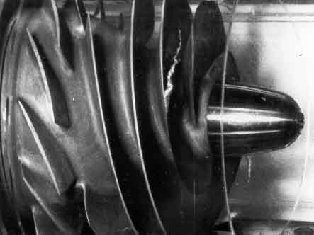
Since cavitation in a pump impeller can take a variety of forms (see, for example, Wood 1963), it is appropriate at this stage to attempt some description and classification of these types of cavitation. It should be borne in mind that any such classification is necessarily somewhat arbitrary, and that types of cavitation may occur that do not readily fall within the classification system. Figure 5.6 includes sketches of some of the forms of cavitation that can be observed in an unshrouded axial flow impeller. As the inlet pressure is decreased, inception almost always occurs in the tip vortex generated by the corner where the leading edge meets the tip. Figure 5.7 includes a photograph of a typical cavitating tip vortex from tests of Impeller IV (the scale model of the SSME low pressure LOX turbopump shown in figure 2.12). Note that the backflow causes the flow in the vicinity of the vortex to have an upstream velocity component. Careful smoothing of the transition from the leading edge to the tip can reduce σi, but it will not eliminate the vortex, or vortex cavitation.
|
| Figure 5.7 Tip vortex cavitation on Impeller IV, the scale model of the SSME low pressure LOX turbopump (see figure 2.12) at an inlet flow coefficient, φ1, of 0.07 and a cavitation number, σ, of 0.42 (from Braisted 1979). |
Usually the cavitation number has to be lowered quite a bit further before the next development occurs, and often this takes the form of traveling bubble cavitation on the suction surfaces of the blades. Nuclei in the inflow grow as they are convected into the regions of low pressure on the suction surfaces of the blades, and then collapse as they move into regions of higher pressure. For convenience, this will be termed ``bubble cavitation.'' It is illustrated in figure 5.8 which shows bubble cavitation on a single hydrofoil.
|
| Figure 5.8 Bubble cavitation on the surface of a NACA 4412 hydrofoil at zero incidence angle, a speed of 13.7 m/s and a cavitation number of 0.3. The flow is from left to right and the leading edge of the foil is just to the left of the white glare patch on the surface (Kermeen 1956). |
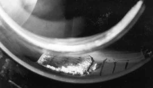
With further reduction in the cavitation number, the bubbles may combine to form large attached cavities or vapor-filled wakes on the suction surfaces of the blades. In a more general context, this is known as ``attached cavitation''. In the context of pumps, it is often called ``blade cavitation''. Figure 5.9 presents an example of blade cavitation in a centrifugal pump.
|
| Figure 5.9 Blade cavitation on the suction surface of a blade in a centrifugal pump. The relative flow is from left to right and the cavity begins at the leading edge of the blade which is toward the left of the photograph. From Sloteman, Cooper, and Graf (1991), courtesy of Ingersoll-Dresser Pump Company. |
When blade cavities (or bubble or vortex cavities) extend to the point on the suction surface opposite the leading edge of the next blade, the increase in pressure in the blade passage tends to collapse the cavity. Consequently, the surface opposite the leading edge of the next blade is a location where cavitation damage is often encountered.
|
| Figure 5.10 Partially cavitating cascade (left) and supercavitating cascade (right). |
|
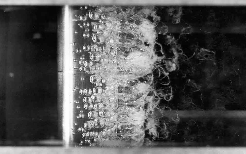
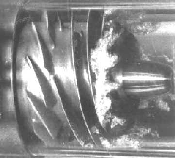
| Figure 5.11 As figure 5.7, but here showing typical backflow cavitation. |
Blade cavitation that collapses on the suction surface of the blade is also referred to as ``partial cavitation'', in order to distinguish it from the circumstances that occur at very low cavitation numbers, when the cavity may extend into the discharge flow downstream of the trailing edge of the blade. These long cavities, which are clearly more likely to occur in lower solidity machines, are termed ``supercavities''. Figure 5.10 illustrates the difference between partial cavitation and supercavitation. Some pumps have even been designed to operate under supercavitating conditions (Pearsall 1963). The potential advantage is that bubble collapse will then occur downstream of the blades, and cavitation damage might thus be minimized.
Finally, it is valuable to create the catch-all term ``backflow cavitation'' to refer to the cavitating bubbles and vortices that occur in the annular region of backflow upstream of the inlet plane when the pump is required to operate in a loaded condition below the design flow rate (see section 4.5). The increased pressure rise across the pump under these circumstances may cause the tip clearance flow to penetrate upstream and generate a backflow that can extend many diameters upstream of the inlet plane. When the pump also cavitates, bubbles and vortices are swept up in this backflow and, to the observer, can often represent the most visible form of cavitation. Figure 5.11 includes a photograph illustrating the typical appearance of backflow cavitation upstream of the inlet plane of an inducer.
|
| Figure 5.12 Histograms of nuclei populations in treated and untreated tap water and the corresponding cavitation inception numbers on hemispherical headforms of three different diameters (Keller 1974). |
In section 5.3 the important role played by cavitation nuclei in determining cavitation inception was illustrated by reference to the comparitive ITTC tests (figure 5.1). It is now clear that measurements of cavitation inception are of little value unless the nuclei population is documented. Unfortunately, this calls into question the value of most of the cavitation inception data found in the literature. And, even more important in the present context, is the fact that this includes just about all of the observations of cavitation inception in pumps. To illustrate this point, we reproduce in figure 5.12 data obtained by Keller (1974) who measured cavitation inception numbers for flows around hemispherical bodies. The water was treated in different ways so that it contained different populations of nuclei, as shown on the left in figure 5.12. As one might anticipate, the water with the higher nuclei population had a substantially larger inception cavitation number.
One of the consequences of this dependence on nuclei population is that it may cause the cavitation number at which cavitation disappears when the pressure is increased (known as the ``desinent'' cavitation number, σd) to be larger than the value at which the cavitation appeared when the pressure was decreased, namely σi. This phenomenon is termed ``cavitation hysteresis'' (Holl and Treaster 1966), and is often the result of the fact mentioned previously (section 5.3) that the cavitation itself can increase the nuclei population in a recirculating facility. An example of cavitation hysteresis in tests on an axial flow pump in a closed loop is given in figure 7.8.
|
| Figure 5.13 Head rise and suction line noise as a function of the Thoma cavitation factor, σTH, for a typical centrifugal pump (adapted from McNulty and Pearsall 1979). |
One of the additional complications is the subjective nature of the judgment that cavitation has appeared. Visual inspection is not always possible, nor is it very objective, since the number of ``events'' (an event is a single bubble growth and collapse) tends to increase over a range of cavitation numbers. If, therefore, one made a judgment based on a certain critical event rate, it is inevitable that the inception cavitation number would increase with nuclei population, as in figure 5.12. Experiments have found, however, that the production of noise is a simpler and more repeatable measure of inception than visual observation. While still subject to the variations with nuclei population, it has the advantage of being quantifiable. Figure 5.13, from McNulty and Pearsall (1979), illustrates the rapid increase in the noise from a centrifugal pump when cavitation inception occurs (the data on inception in figure 5.5 and table 5.1 was obtained acoustically).
|
| Figure 5.14 The effect of air content on the critical cavitation numbers for a centrifugal pump (Schoeneberger 1965, Pearsall 1972). |
Though information on the nuclei are missing in most experiments, the total air content of the water is frequently monitored. One would suppose that the nuclei population would increase with the air content, and this is usually the case. Some data on the dependence of the critical cavitation numbers for a centrifugal pump on the total air content is included in figure 5.14. As expected, the cavitation inception number, σi, increases with air content. Note, however, that the breakdown cavitation number, σb, is quite independent of air content, an illustration of the fact that, once it has been initiated, cavitation is much less dependent on the nuclei population.
|
| Figure 5.15 Cavitation inception characteristics of a NACA 4412 hydrofoil (Kermeen 1956). |
Having begun by questioning the value of much of the cavitation inception data, we will nevertheless proceed to review some of the important trends in that data base. In doing so we might take refuge in the thought that each investigator probably applied a consistent criterion in assessing cavitation inception, and that the nuclei content in a given facility might be fairly constant (though the latter is very doubtful). Then, though the data from different investigators and facilties may be widely scattered, one would hope that the trends exhibited in a particular research project would be qualitatively significant.
Consider first the inception characteristics of a single hydrofoil as the angle of incidence is varied. Typical data, obtained by Kermeen (1956) for a NACA 4412 hydrofoil, is reproduced in figure 5.15. At positive angles of incidence, the regions of low pressure and cavitation inception will occur on the suction surface; at negative angles of incidence, these phenomena will shift to what is normally the pressure surface. Furthermore, as the angle of incidence is increased in either direction, the value of -Cpmin will increase, and hence the inception cavitation number will also increase.
|
| Figure 5.16 Calculated cavitation inception number, σi (or -Cpmin), as a function of blade angle, βb1, solidity, s, and incidence angle, α, for a cascade of NACA-65-010 hydrofoils (Herrig et al. 1957, Pearsall 1972). |
When such hydrofoils are used to construct a cascade, the results will also depend on the cascade solidity, s. Data on the pressure distributions around a blade in a cascade (such as that of Herrig et al. 1957) can be used to determine Cpmin as a function of blade angle, βb1, solidity, s, and angle of incidence, α. Consequently, one can anticipate the variation in the inception number with these variables, assuming the first-order approximation, σi= -Cpmin. An example of such data is presented in figure 5.16; this was derived by Pearsall (1972) from the cascade data of Herrig et al. (1957). Note that a particular cascade will have a particular positive angle of incidence of, typically, a few degrees, at which σi is a minimum. The optimum angle of incidence changes with different s and βb1; however, it seems to lie within a fairly narrow range between 1 and 5 degrees for a wide range of those design variables. In a pump, the incidence angle is usually small in the vicinity of the design flow rate, but will increase substantially above or below the design value. Consequently, in a pump, the cavitation inception number tends to have a minimum at the design flow rate. This is illustrated in figure 5.17 which includes some data from a typical centrifugal pump, and by the data in figure 7.7 for an axial flow pump.
|
| Figure 5.17 Variation in the inception number with flow rate for a typical centrifugal pump (adapted from McNulty and Pearsall 1979). |
|
| Figure 5.18 The desinent cavitation numbers for three geometrically similar Joukowski hydrofoils at zero angle of incidence as a function of Reynolds number, Uc/ν (Holl and Wislicenus 1961). Note the theoretical Cpmin=-0.54. |
As discussed in section 5.4, the scaling of cavitation phenomena with size and with speed can be an important issue. Typical data for cavitation inception on a single hydrofoil is that obtained by Holl and Wislicenus (1961); it is reproduced in figure 5.18. Data for three different sizes of 12% Joukowski hydrofoil (at zero angle of incidence) were obtained at different speeds. It was plotted against Reynolds number in the hope that this would reduce the data to a single curve. The fact that this does not occur demonstrates that there is a size or speed effect separate from that due to the Reynolds number. It seems plausible that the missing parameter is the ratio of the nuclei size to chord length; however, in the absence of information on the nuclei, such a conclusion is speculative.
To complete the list of those factors that may influence cavitation inception, it is necessary to mention the effects of surface roughness and of the turbulence level in the flow. The two effects are connected to some degree, since roughness will affect the level of turbulence. But roughness can also affect the flow by delaying boundary layer separation and therefore modifying the pressure and velocity fields in a more global manner. The reader is referred to Arndt and Ippen (1968) for details of the effects of surface roughness on cavitation inception.
Turbulence affects cavitation inception since a nucleus may find itself in the core of a vortex where the pressure level is lower than the mean. It could therefore cavitate when it might not do so under the influence of the prevailing mean pressure level. Thus turbulence may promote cavitation, but one must also allow for the fact that it may alter the global pressure field by altering the location of flow separation. These complicated viscous effects on cavitation inception were first examined in detail by Arakeri and Acosta (1974) and Gates and Acosta (1978) (see also Arakeri 1979). The implications for cavitation inception in the highly turbulent environment of most pump flows have yet to be examined in detail.
|
| Figure 5.19 The cavitation inception number, σi, as a function of tip clearance, δ (τmax is the maximum blade thickness), in an unshrouded axial flow pump at various flow coefficients, φ (adapted from Rains 1954). |
|
| Figure 5.20 The cavitation inception number as a function of radial tip clearance in an axial inducer (Janigro and Ferrini 1973 from data of Acosta 1958 and Henderson and Tucker 1962). |
In unshrouded turbomachinery, cavitation usually begins in the vortices associated with the tip clearance flows, and so it is important to investigate how the tip clearance will affect the inception number. In figures 5.19 and 5.20 observed cavitation inception numbers for the tip clearance flows in axial flow impellers are plotted against nondimensional tip clearance. The typical variation with incidence angle or flow coefficients is illustrated in figure 5.19 (Rains 1954). Since the pressure difference between the two sides of the blade increases with incidence angle, the velocities of the tip clearance flow must also increase, and it follows that σi should increase correspondingly, as is the case in figure 5.19. A second feature that is not clear in Rains' data, but is manifest in the data of Acosta (1958) and Henderson and Tucker (1962), is that there appears to be an optimum tip clearance of about 1% of the blade height. At this optimum, the cavitation inception number is a minimum. This is illustrated in the figure 5.20.
- Acosta, A.J. (1958). An experimental study of cavitating inducers. Proc. Second ONR Symp. on Naval Hydrodynamics, ONR/ACR-38, 533--557.
- Acosta, A.J. and Parkin, B.R. (1975). Cavitation inception---a selective review. J. Ship Res., 19, No. 4, 193--205.
- Arakeri, V.H. and Acosta, A.J. (1974). Viscous effects in the inception of cavitation on axisymmetric bodies. ASME J. Fluids Eng., 95, No. 4, 519--528.
- Arakeri, V.H. (1979). Cavitation inception. Proc. Indian Acad. Sci., C2, Part 2, 149--177.
- Arndt, R.E.A. and Ippen, A.T. (1968). Rough surface effects on cavitation inception. ASME J. Basic Eng., 90, 249--261.
- Arndt, R.E.A. and Keller, A.P. (1976). Free gas content effects on cavitation inception and noise in a free shear flow. Proc. IAHR Symp. on two-phase flow and cavitation in power generation, 3--16.
- Billet, M.L. (1985). Cavitation nuclei measurements---a review. Proc. 1985 Cavitation and Multiphase Flow Forum, FED 23, 31--38.
- Braisted, D.M. (1979). Cavitation induced instabilities associated with turbomachines. Ph.D. Thesis, California Institute of Technology, Pasadena, Ca.
- Brennen, C.E. (1994). Cavitation and bubble dynamics. Oxford Univ. Press.
- Gates, E.M. and Acosta, A.J. (1978). Some effects of several free stream factors on cavitation inception on axisymmetric bodies. Proc. 12th ONR Symp. on Naval Hydrodynamics, 86--108.
- Gavrilov, L.R. (1970). Free gas content of a liquid and acoustical techniques for its measurement. Sov. Phys.---Acoustics, 15, No.3, 285--295.
- Henderson and Tucker (1962). Performance investigation of some high speed pump inducers. R.P.E. Tech. Note 214. Referred to by Janigro and Ferrini (1973) but not located by the author.
- Herrig, L.J., Emery, J.C., and Erwin, J.R. (1957). Systematic two-dimensional cascade tests of NACA 65-series compressor blades at low speeds. NACA TN 3916.
- Holl, J.W. and Wislicenus, G.F. (1961). Scale effects on cavitation. ASME J. Basic Eng., 83, 385--398.
- Holl, J.W. and Treaster, A.L. (1966). Cavitation hysteresis. ASME J. Basic Eng., 88, 199--212.
- Hydraulic Institute, New York. (1965). Standards of the Hydraulic Institute (11th edition).
- Janigro, A. and Ferrini, F. (1973). Inducer pumps. In Recent progress in pump research, von Karman Inst. for Fluid Dynamics, Lecture Series 61.
- Johnsson, C.A. (1969). Cavitation inception on headforms, further tests. Proc. 12th Int. Towing Tank Conf., Rome, 381--392.
- Katz, J., Gowing, S., O'Hern, T., and Acosta, A.J. (1984). A comparitive study between holographic and light-scattering techniques of microbubble detection. Proc. IUTAM Symp. on Measuring Techniques in Gas-Liquid Two-Phase Flows, Springer-Verlag, 41--66.
- Keller, A.P. (1974). Investigations concerning scale effects of the inception of cavitation. Proc. I.Mech.E. Conf. on Cavitation, 109--117.
- Keller, A.P. and Weitendorf, E.A. (1976). Influence of undissolved air content on cavitation phenomena at the propeller blades and on induced hull pressure amplitudes. Proc. IAHR Symp. on two-phase flow and cavitation in power generation, 65--76.
- Kermeen, R.W. (1956). Water tunnel tests of NACA 4412 and Walchner Profile 7 hydrofoils in noncavitating and cavitating flows. Calif. Inst. of Tech., Hydrodynamics Lab. Rep. 47-5.
- Knapp, R.T., Daily, J.W., and Hammitt, F.G. (1970). Cavitation. McGraw-Hill, New York.
- Lindgren, H. and Johnsson, C.A. (1966). Cavitation inception on headforms, ITTC comparative experiments. Proc. 11th Int. Towing Tank Conf., Tokyo, 219--232.
- McNulty, P.J. and Pearsall, I.S. (1979). Cavitation inception in pumps. ASME Int. Symp. on Cavitation Inception, 163--170.
- Medwin, H. (1977). In situ acoustic measurements of microbubbles at sea. J. Geophys. Res., 82, No.6, 921--976.
- Pearsall, I.S. (1963). Supercavitation for pumps and turbines. Engineering (GB), 196(5081), 309--311.
- Pearsall, I.S. (1972). Cavitation. Mills & Boon Ltd., London.
- Peterson, F.B., Danel, F., Keller, A.P., and Lecoffre, Y. (1975). Determination of bubble and particulate spectra and number density in a water tunnel with three optical techniques. Proc. 14th Int. Towing Tank Conf., Ottawa, 2, 27--52.
- Rains, D.A. (1954). Tip clearance flows in axial flow compressors and pumps. Calif. Inst. of Tech. Hydro. and Mech. Eng. Lab. Report, No. 5.
- Schoeneberger, W. (1965). Cavitation tests in radial pump impellers. Ph.D. Thesis, Tech. Univ. Darmstadt.
- Sloteman, D.P., Cooper, P., and Graf, E. (1991). Design of high-energy pump impellers to avoid cavitation instabilities and damage. Proc. EPRI Power Plant Symp., Tampa, Fl., June 1991.
- Wood, G.M. (1963). Visual cavitation studies of mixed flow pump impellers. ASME J. Basic Eng., Mar. 1963, 17--28.
Last updated 12/1/00.
Christopher E. Brennen