HYDRODYNAMICS OF PUMPS
by Christopher Earls Brennen © Concepts NREC 1994
CHAPTER 4.
OTHER FLOW FEATURES
4.1 INTRODUCTION
In this chapter we briefly survey some of the other important features of the flows through turbomachines. We begin with a section on the three-dimensional characteristics of flows, and a discussion of some of the difficulties encountered in adapting the cascade analyses of the last chapter to the complex geometry of most turbomachines.
4.2 THREE-DIMENSIONAL FLOW EFFECTS
|
| Figure 4.1 Geometry of a meridional streamtube in a pump impeller. |
The preceding chapter included a description of some of the characteristics of two-dimensional cascade flows in both the axial and radial geometries. It was assumed that the flow in the meridional plane was essentially two-dimensional, and that the effects of the velocities (and the gradients in the velocity or pressure) normal to the meridional surface were neglible. Moreover, it was tacitly assumed that the flow in a real turbomachine could be synthesized using a series of these two-dimensional solutions for each meridional annulus. In doing so it is implicitly assumed that each annulus corresponds to a streamtube such as depicted in figure 4.1 and that the geometric relations between the inlet location, r1, and thickness, dr1, and the discharge thickness, dn, and location, r2, are known a priori. In practice this is not the case and quasi-three-dimensional methods have been developed in order to determine the geometrical relation, r2(r1). These methods continue to assume that the streamsurfaces are axisymmetric, and, therefore, neglect the more complicated three-dimensional aspects of the flow exemplified by the secondary flows discussed below (section 4.6). Nevertheless, these methods allow the calculation of useful turbomachine performance characteristics, particularly under circumstances in which the complex secondary flows are of less importance, such as close to the design condition. When the turbomachine is operating far from the design condition, the flow within a blade passage may have streamsurfaces that are far from axisymmetric.
In the context of axial flow machines, several approximate methods have been employed in order to determine r2(r1) as a part of a quasi-three-dimensional solution to the flow. Most of these are based on some application of the condition of radial equilibrium. In its simplest form, the radial equilibrium condition assumes that all of the terms in the equation of motion normal to the axisymmetric streamsurface are negligible, except for the pressure gradient and the centrifugal acceleration terms, so that
 | ......(4.1) |
The following example will illustrate one use of the ``radial equilibrium'' condition. We shall assume that the inlet flow is in radial equilibrium. This inlet flow is then divided into axisymmetric streamtubes, each with a specific radial location, r1. Some initial estimate is made of the radial location of each of the streamtubes at discharge (in other words an estimate of the function r2(r1)). Then an iterative numerical method is employed, in which the total pressure rise through each streamtube is evaluated. Hence, the pressure distribution at discharge can be obtained. Then the width of each tube at discharge is adjusted (r2(r1) is adjusted) in order to obtain the required radial pressure gradient between each pair of adjacent streamtubes. Subsequently, the process is repeated until a converged solution is reached. In some simple cases, analytical rather than numerical results can be obtained; an example is given in the next section.
More generally, it should be noted that quasi-three-dimensional analyses of this kind are often used for the design of axial turbomachines. A common objective is to achieve a design in which the total pressure is increasing (or decreasing) with axial position at the same rate at all radii, and, therefore, should be invariant with radial position. Combining this with the condition for radial equilibrium, leads to
 | ......(4.2) |
|
| Figure 4.2 Actuator disc model of an axial blade row with a generic meridional streamtube. |
Radial equilibrium of the discharge flow may be an accurate assumption in some machines but not in others. When the blade passage is narrow (in both directions) relative to its length, the flow has adequate opportunity to adjust within the impeller or rotor passage, and the condition of radial equilibrium at discharge is usually reasonable. This is approximately the case in all pumps except propeller pumps of low solidity. However, in many compressors and turbines, the blade height is large compared with the chord and a radial equilibrium assumption at discharge is not appropriate. Under these circumstances, a very different approach utilizing an ``actuator disc'' has been successfully employed. The flows far upstream and downstream of the blade row are assumed to be in radial equilibrium, and the focus is on the adjustment of the flow between these locations and the blade row (see figure 4.2). The flow through the blade row itself is assumed to be so short that the streamsurfaces emerge at the same radial locations at which they entered; thus the blade row is modeled by an infinitesmally thin ``actuator disc''. In some respects, the actuator disc approach is the opposite of the radial equilibrium method; in the former, all the streamline adjustment is assumed to occur external to the blade passages whereas, in many radial equilibrium applications, the adjustment all occurs internally.
Since actuator disc methods are rarely applied in the context of pumps we shall not extend the discussion of them further. More detail can be found in texts such as Horlock (1973). We shall, however, provide an example of a radial equilibrium analysis since the results will prove useful in a later chapter.
4.3 RADIAL EQUILIBRIUM SOLUTION: AN EXAMPLE
For the purposes of this example of a radial equilibrium solution, the flow through the pump impeller is subdivided into streamtubes, as shown in figure 4.1. We choose to examine one generic streamtube with an inlet radius, r1, and thickness, dr1. Both the position, n, and the thickness, dn, of the streamtube at discharge are not known a priori, and must be determined as a part of the solution. Conservation of mass requires that
 | ......(4.3) |
 .
.
Applying the radial equilibrium assumption, the pressure distribution over the exit plane is given by
 | ......(4.4) |
=0, and a constant βb2 in the case of
a centrifugal pump with =90°. Moreover, we shall assume that
the flow at discharge is parallel with the blades so that β2(n)
=βb2(n).
The formulation of the problem is now complete, and it is a relatively straightforward matter to eliminate p2(n) from equations 2.30 and 4.4, and then use the velocity triangles and the continuity equation 4.3 to develop a single differential equation for vm2(n). Assuming that the inlet is free of swirl, and that vm1 is a constant, this equation for vm2(n) can then be integrated to obtain the velocity and pressure distributions over the exit. It remains to evaluate the total energy added to the flow by summing the energies added to each of the streamtubes according to equation 2.21:
 | ......(4.5) |
 | ......(4.6) |
 | ......(4.7) |
 | ......(4.8) |
Examples of these analytical performance curves are given later in figures 7.13 and 7.15. Note that this idealized hydraulic performance is a function only of the geometric variables, Γ and βbT2, of the discharge. Moreover, it is readily shown that in the centrifugal limit of Γ→ 0 then Σ1→ 1, Σ2→ -cot βbT2, Σ3→ 0, and the earlier result of equation 2.33 is recovered.
It is of interest to explore some optimizations based on the hydraulic performance, given by equation 4.6. Though the arguments presented here are quite heuristic, the results are interesting. We begin with the observation that two particular geometric factors are important in determining the viscous losses in many internal flows. If the cross-sectional area of the flow increases at more than a marginal rate, the deceleration-induced boundary layer separation and turbulence can lead to large viscous losses that might not otherwise occur. Consequently, the mean value of w2/w1 is an important design parameter, as implied earlier in section 3.4. In the present analysis, the mean value of this parameter is given by the area ratio, Ar*, where, from geometric considerations,
 | ......(4.9) |
 | ......(4.10) |
Many centrifugal pumps are designed with Ar* values somewhat greater than unity because the flow must subsequently be decelerated in the diffuser and volute, and smaller values of Ar* would imply larger diffusion losses in those nonrotating components. But, from the point of view of minimizing losses in the impeller alone, one justifiable optimization would require Ar* to be approximately unity.
The second geometric factor that can influence the magnitude of the viscous losses in an internal flow is the amount of turning imposed on the flow. In the present analysis, we shall make use of an angle, ε, describing the ``angle of turn'' of the flow as it proceeds through the turbomachine. It is defined as the angle of the discharge relative velocity vector to the conical discharge surface minus the angle of the inlet relative velocity vector to the inlet surface:
 | ......(4.11) |
|
| Figure 4.3 Comparison of the results of equation 4.14 with the conventional recommendation from figure 2.7 for the optimum ratio of inlet to discharge tip radius as a function of design specific speed, ND. |
|
| Figure 4.4 Comparison of the results of equation 4.14 with the conventional recommendation of figure 2.7 for the head coefficient, ψD, and the flow coefficient, φD, as functions of the design specific speed, ND. |
For the purposes of this example, we now postulate that the major hydraulic losses encountered in the flow through the pump are minimized when ε is minimized. Let us assume that this minimum value of ε can be approximated by zero. Referring to this maximum efficiency point of operation as the ``design point'' (where conditions are denoted by the suffix, D), it follows from equation 4.11 that
 | ......(4.12) |
 | ......(4.13) |
 | ......(4.14) |
, and βbT2.
Examine now the variation of ND with these geometric variables, as manifest
by equation 4.14, bearing in mind that the practical design problem involves
the reverse procedure of choosing the geometry best suited to a known
specific speed. The number of geometric variables will be reduced to four
by assuming RH1=0. Note also that, at the design point given by
equation 4.12, it follows that Ar*=Ar and it is more convenient
to use this area ratio in place of the variable RH2/RT2. Thus we
consider the
variations of ND with , βbT2, RT1/RT2, and Ar*.
Calculations of ND from equation 4.14 show that, for specific speeds
less than unity, for sensible values of Ar* of the order of unity, and
for blade angles βbT2 which are less than
about 70° (which is the case in
well-designed pumps), the results are virtually independent of the angle
, a feature that simplifies the parametric
variations in the results. For convenience, we choose an arbitrary value of
=50°. Then typical results for Ar*=1.0 are presented in
figure 4.3, which shows
the ``optimum'' RT1/RT2 for various design
specific speeds, ND, at various discharge blade angles, βbT2.
Considering the heuristic nature of some of the assumptions that were
used in this optimization, the agreement between the results and
the conventional recommendation (reproduced from figure 2.7) is remarkable.
It suggests that the evolution of pump designs has been driven
by processes minimizing the viscous losses, and that this minimization
involves the optimization of some simple geometric variables.
The values of ψD and φD, that correspond to the results of
figure 4.3, are plotted in figure 4.4.
Again, the comparison of the traditional
expectation and the present analysis is good, except perhaps at low
specific speeds where the discrepancy may be due to the large values of
Ar* which are used in practice. Finally, we observe that one can
construct sets of curves, such as those of figure 4.3, for other values of the
area ratio, Ar*. However, for reasonable values of βbT2 like
20°,
the curves for 0.8 < Ar* < 2.0 do not differ greatly from those
for Ar*=1.0.
The foregoing analysis is intended only as an example of the application of the radial equilibrium methodology, and the postscript is included because of the interesting results it produces. Clearly some of the assumptions in the postscript are approximate, and would be inappropriate in any accurate analysis of the viscous losses.
To this point the entire focus has been on the flow within the impeller or rotor of the pump. However, the flow that discharges from the impeller requires careful handling in order to preserve the gains in energy imparted to the fluid. In many machines this requires the conversion of velocity head to pressure by means of a diffuser. This inevitably implies hydraulic losses, and considerable care needs to be taken to minimize these losses. The design of axial and radial diffusers, with and without vanes to recover the swirl velocity, is a major topic, whose details are beyond the scope of this book. The reader is referred to the treatise by Japikse (1984).
Such diffusers are more common in compressors than in pumps. Typical pump configurations are as follows. Axial flow pumps often employ a set of stator vanes before (or in) the axial diffuser in order to recover the swirl velocities. Special care needs to be taken to match the swirl angles of the flow exiting the impeller with the inlet angles of the stator vanes. It is advisable, where possible, to measure the impeller discharge flow directly before finalizing a design. In some designs, the axial diffuser will be followed by a spiral collector or ``volute'' in order to recover the energy in the remaining swirl and axial velocities.
|
| Figure 4.5 Volute flow notation. |
In the case of centrifugal pumps, a radial flow diffuser with vanes may or may not be used. Often it is not, and the flow discharges directly into the volute. The proper design of this volute is an important component of centrifugal pump design (Anderson 1955, Worster 1963, Stepanoff 1948). The objective is to design a volute in which the flow is carefully matched to the flow exiting the impeller, so that the losses are minimized and so that the pressure is uniform around the impeller discharge. The basic concept is sketched in figure 4.5. The flow discharges from the impeller with a velocity, vθ2, in the tangential direction and a velocity, vr2, in the radial direction, given by
 | ......(4.15) |
If we further assume radially uniform velocity at each angular location in the volute (also an assumption that needs to be modified in a more accurate analysis), then it follows from the application of conservation of mass to an element, dθ, of the volute that the discharge flow will be matched to the flow in the volute if
 | ......(4.16) |
 | ......(4.17) |
 | ......(4.18) |
Consequently, for a given impeller operating at a given design flow coefficient, φD, there exists a specific area ratio, 2π R2 B2 tanβ2/AVT, for the volute geometry. This parameter is close to the ratio which Anderson (1955) used in his design methodology (see also Worster 1963), namely the ratio of the cross-sectional area of the flow leaving the impeller (2π R2B2sinβ2) to the volute throat area (AVT). For more detailed analyses of the flow in a volute, the reader is referred to Pfleiderer (1932), Stepanoff (1948), and Lazarkiewicz and Troskolanski (1965). For example, Pfleiderer explored the radially nonuniform distributions of velocity within the volute and the consequences for the design methodology.
One of the other considerations during the design of a volute is the lateral force on the impeller that can develop due to circumferentially nonuniform flow and pressure in the volute. These, and other related issues, are discussed in chapter 10.
4.5 PREROTATION
Perhaps no aspect of turbomachinery flow is more misrepresented and misunderstood than the phenomenon of ``prerotation''. While this belongs within the larger category of secondary flows (dealt with in section 4.6), it is appropriate to address the issue of prerotation seperately, not only because of its importance for the hydraulic performance, but also because of its interaction with cavitation.
It is first essential to distinguish between two separate phenomena both of which lead to a swirling flow entering the pump. These two phenomena have very different fluid mechanical origins. Here we shall distinguish them by the separate terms, ``backflow-induced swirl'' and ``inlet prerotation''. Both imply a swirl component of the flow entering the pump. In fluid mechanical terms, the flow has axial vorticity (if the axis of rotation is parallel with the axis of the inlet duct) with a magnitude equal to twice the rate of angular rotation of the swirl motion. Moreover, there are some basic properties of such swirling flows that are important to the understanding of prerotation. These are derived from the vorticity transport theorem (see, for example, Batchelor 1967). In the context of the steady flow in an inlet duct, this theorem tells us that the vorticity will only change with axial location for two reasons: (a) because vorticity is diffused into the flow by the action of viscosity, or (b) because the flow is accelerated or decelerated as a result of a change in the cross-sectional area of the flow. The second mechanism results in an increase in the swirl velocity due to the stretching of the vortex line, and is similar to the increase in rotation experienced by figure skaters when they draw their arms in closer to their body. When the moment of inertia is decreased, conservation of angular momentum results in an increase in the rotation rate. Thus, for example, a nozzle in the inlet line would increase the magnitude of any preexisting swirl.
For simplicity, however, we shall first consider inlet ducting of uniform and symmetric cross-sectional area, so that only the first mechanism exists. In inviscid flow, it follows that, if there is a location far upstream at which the swirl (or axial vorticity) is zero, then, in the absence of viscous effects, the swirl will be everywhere zero. This important result, which is a version of Kelvin's theorem (Batchelor 1967), is not widely recognized in discussions of prerotation. Moreover, the result is not altered by the existence of viscous effects, since purely axial motion cannot generate axial vorticity. However, there are two common circumstances in which prerotation can be generated without violation of the above theorem, and these give rise to the two phenomena named earlier.
|
| Figure 4.6 Lateral view of impeller inlet flow showing tip leakage flow leading to backflow. |
The first of these common circumstances arises because of one of the most important secondary flows that can occur in pumps, namely the phenomenon of ``backflow''. This is caused by the leakage flow between the tip of the blades of an impeller (we consider first an unshrouded impeller) and the pump casing. The circumstances are depicted in figure 4.6. Below a certain critical flow coefficient, the pressure difference driving the leakage flow becomes sufficiently large that the tip leakage jet penetrates upstream of the inlet plane of the impeller, and thus forms an annular region of ``backflow'' in the inlet duct. After penetrating upstream a certain distance, the fluid of this jet is then entrained back into the main inlet flow. The upstream penetration distance increases with decreasing flow coefficient, and can reach many diameters upstream of the inlet plane. In some pump development programs (such as the Rocketdyne J-2 liquid oxygen pump) efforts have been made to insert a ``backflow deflector'' in order to improve pump performance (Jakobsen 1971). The intention of such a device is to prevent the backflow from penetrating too far upstream, to reduce the distortion of the inlet flow field, and to recover, as far as is possible, the swirl energy in the backflow. More recently, a similar device was successfully employed in a centrifugal pump (Sloteman et al. 1984).
|
| Figure 4.7 Axial and swirl velocity profiles in the inlet duct 0.25 diameters (left) and 0.5 diameters (right) upstream of the inlet plane of an inducer (Impeller VI) for various flow coefficients as shown (from del Valle, Braisted and Brennen 1992). |
Some measurements of the axial and swirl velocities just upstream of an axial inducer are presented in figure 4.7. This data is taken from del Valle et al (1992), though very similar velocity profiles have been reported by Badowski (1969, 1970) (see also Janigro and Ferrini 1973), and the overall features of the flow are similar whether the pump is shrouded or unshrouded, axial or centrifugal (see, for example, Stepanoff 1948, Okamura and Miyashiro 1978, Breugelmans and Sen 1982, Sloteman et al. 1984). Measurements are shown in figure 4.7 for two distances upstream of the inlet plane (half a radius and one radius upstream), and for a number of flow coefficients, φ. Note from the axial flow velocity profiles that, as the flow coefficient is decreased, the backflow reaches a half radius upstream at a flow coefficient, φ of about 0.066, and one radius upstream at about 0.063. The size of the backflow region grows as φ is decreased. It is particularly remarkable that at a flow coefficient of 0.05, nearly 30% of the inlet area is experiencing reverse flow! We can further observe from the swirl velocity data that, in the absence of backflow, the inlet flow has zero swirl. Kelvin's theorem tells us this must be the case because the flow far upstream has no swirl.
Obviously the backflow has a high swirl velocity imparted to it by the impeller blades. But what is also remarkable is that this vorticity is rapidly spread to the core of the main inlet flow, so that at φ=0.05, for example, almost the entire inlet flow has a nonzero swirl velocity. The properties of swirling flows discussed above are not violated, since the origin of the vorticity is the pump itself and the vorticity is transmitted to the inflow via the backflow. The rapidity with which the swirl vorticity is diffused to the core of the incoming flow remains something of a mystery, for it is much too rapid to be caused by normal viscous diffusion (Braisted 1979). It seems likely that the inherent unsteadiness of the backflow (with a strong blade passing frequency component) creates extensive mixing which effects this rapid diffusion. However it arises, it is clear that this ``backflow-induced swirl'', or ``pre-rotation'', will clearly affect the incidence angles and, therefore, the performance of the pump.
Before leaving the subject of backflow, it is important to emphasize that this phenomenon also occurs at flow rates below design in centrifugal as well as axial flow pumps, and with shrouded as well as unshrouded impellers (see, for example, Okamura and Miyashiro 1978, Makay 1980). The detailed explanation may differ from one device to another, but the fundamental tendency for an impeller to exhibit this kind of secondary flow at larger angles of incidence seems to be universal.
|
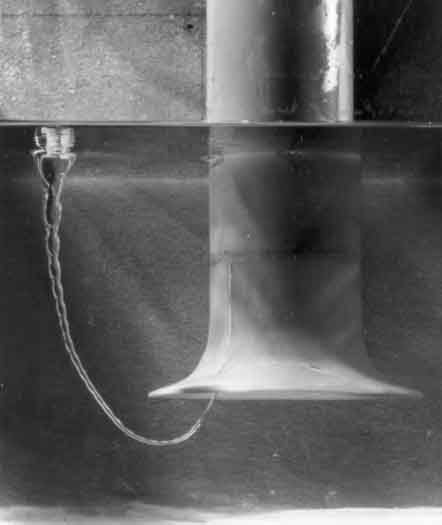
| Figure 4.8 Right: sketch of a typical inlet vortex associated with prerotation. Left: Photograph of an air-filled inlet vortex from Wijdieks (1965) reproduced with permission of the Delft Hydraulics Laboratory. |
But there is another, quite separate origin for prerotation, and this is usually manifest in practice when the fluid is being drawn into the pump from an ``inlet bay'' or reservoir with a free surface (figure 4.8). Under such circumstances, it is almost inevitable that the large scale flow in the reservoir has some nonuniformity that constitutes axial vorticity or circulation in the frame of reference of the pump inlet. Even though the fluid velocities associated with this nonuniformity may be very small, when the vortex lines are stretched as the flow enters the inlet duct, the vorticity is greatly amplified, and the inlet flow assumes a significant preswirl or ``inlet prerotation''. The effect is very similar to the bathtub vortex. Once the flow has entered an inlet duct of constant cross-sectional area, the magnitude of the swirl usually remains fairly constant over the short lengths of inlet ducting commonly used.
Often, the existence of ``inlet prerotation'' can have unforeseen consequences for the suction performance of the pump. Frequently, as in the case of the bathtub vortex, the core of the vortex runs from the inlet duct to the free surface of the reservoir, as shown in figure 4.8. Due to the low pressure in the center of the vortex, air is drawn into the core and may even penetrate to the depth of the duct inlet, as illustrated by the photograph in figure 4.8 taken from the work of Wijdieks (1965). When this occurs, the pump inlet suddenly experiences a two-phase air/water flow rather than the single-phase liquid inlet flow expected. This can lead, not only to a significant reduction in the performance of the pump, but also to the vibration and unsteadiness that often accompany two-phase flow. Even without air entrainment, the pump performance is almost always deteriorated by these suction vortices. Indeed this is one of the prime suspects when the expected performance is not realized in a particular installation. These intake vortices are very similar to those which can occur in aircraft engines (De Siervi et al. 1982).
|
| Figure 4.9 Cross-section of a blade passage in an axial flow impeller showing the tip leakage flow, boundary layer radial flow, and other secondary flows (adapted from Lakshminarayana 1981). |
Most pumps operate at high Reynolds numbers, and, in this regime of flow, most of the hydraulic losses occur as a result of secondary flows and turbulent mixing. While a detailed analysis of secondary flows is beyond the scope of this monograph (the reader is referred to Horlock and Lakshminarayana (1973) for a review of the fundamentals), it is important to outline some of the more common secondary flows that occur in pumps. To do so, we choose to describe the secondary flows associated with three typical pump components, the unshrouded axial flow impeller or inducer, the shrouded centrifugal impeller, and the vaneless volute of a centrifugal pump.
|
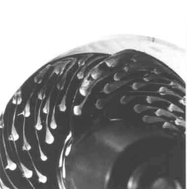
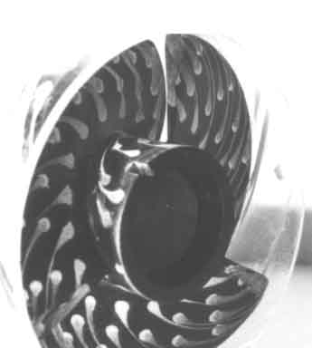
| Figure 4.10 Photographs of a 10.2cm, 12° helical inducer with a lucite shroud showing the blade surface flow revealed by the running paint dot technique. On the left the suction surfaces viewed from the direction of the inlet. On the right the view of the pressure surfaces and the hub from the discharge. The flow is for 2000 rpm and φ1=0.041. From Bhattacharyya et al. (1993). |
Secondary flows in unshrouded axial flow inducers have been studied in detail by Lakshminarayana (1972, 1981), and figure 4.9, which was adapted from those publications, provides a summary of the kinds of secondary flows that occur within the blade passage of such an impeller. Dividing the cross-section into a core region, boundary layer regions on the pressure and suction surfaces of the blades, and an interference region next to the static casing, Lakshminarayana identifies the following departures from a simple flow following the blades. First, and perhaps most important, there will be a strong leakage flow (called the tip leakage or tip clearance flow) around the blade tips driven by the pressure difference between the pressure surface and the suction surface. Clearly this flow will become even more pronounced at flow rates below design when the blades are more heavily loaded. This leakage flow will entrain secondary flow on both surfaces of the blades, as shown by the dashed arrows in figure 4.9.
|
| Figure 4.11 Schematic showing secondary flows associated with a typical centrifugal pump operating at off-design conditions (adapted from Makay 1980). |
Second, the flow in the boundary layers will tend to generate an outward radial component on both the suction and pressure surfaces, though the former may be stronger because of enhancement by the leakage flow. The photographs of figure 4.10, which are taken from Bhattacharyya et al. (1993), show a strong outward radial component of the flow on the blade surface of an inducer. This is particularly pronounced near the leading edge (left-hand photograph). Incidentally, Bhattacharyya et al. not only observed the backflow associated with the tip clearance flow, but also a ``backflow'' at the hub in which flow reenters the blade passage from downstream of the inducer. Evidence for this secondary flow can be seen on the hub surface in the right-hand photograph of figure 4.10. Finally, we should mention that Lakshminarayana also observed secondary vortices at both the hub and the casing as sketched in figure 4.9. The vortex near the hub was larger and more coherent, while a confused interference region existed near the casing.
|
| Figure 4.12 Schematic of a centrifugal pump with a single, vaneless volute indicating the disturbed and separated flows which can occur in the volute below (left) and above (right) the design flow rate. |
Additional examples of secondary flows are given in the descriptions by Makay (1980) of typical flows through shrouded centrifugal impellers. Figure 4.11, which has been adapted from one of Makay's sketches, illustrates the kind of secondary flows that can occur at off-design conditions. Note, in particular, the backflow in the impeller eye of this shrouded impeller pump. This backflow may well interact in an important way with the discharge-to-suction leakage flow that is an important feature of the hydraulics of a centrifugal pump at all flow rates. As testament to the importance of the backflow, Makay cites a case in which the inlet guide vanes of a primary coolant pump in a power plant suffered structural damage due to the repeated unsteady loads caused by this backflow. Note should also be made of the secondary flows that Makay describes occurring in the vicinity of the impeller discharge.
It is also important to mention the disturbed and separated flows that can often occur in the volute of a centrifugal pump when that combination is operated at off-design flow rates (Binder and Knapp 1936, Worster 1963, Lazarkiewicz and Troskolanski 1965, Johnston and Dean 1966). As described in the preceding section, and as indicated in figure 4.12, one of the commonest geometries is the spiral volute, designed to collect the flow discharging from an impeller in a way that would result in circumferentially uniform pressure and velocity. However, such a volute design is specific to a particular design flow coefficient. At flow rates above or below design, disturbed and separated flows can occur particularly in the vicinity of the cutwater or tongue. Some typical phenomena are sketched in figure 4.12 which shows separation on the inside and outside of the tongue at flow coefficients below and above design, respectively. It also indicates the flow reversal inside the tongue that can occur above design (Lazarkiewicz and Troskolanski 1965). Moreover, as Chu et al. (1993) have recently demonstrated, the unsteady shedding of vortices from the cutwater can be an important source of vibration and noise.
- Anderson, H.H. (1955). Modern developments in the use of large single-entry centrifugal pumps. Proc. Inst. Mech. Eng., 169, 141--161.
- Badowski, H.R. (1969). An explanation for instability in cavitating inducers. Proc. 1969 ASME Cavitation Forum, 38--40.
- Badowski, H.R. (1970). Inducers for centrifugal pumps. Worthington Canada, Ltd., Internal Report.
- Batchelor, G.K. (1967). An introduction to fluid dynamics. Cambridge Univ. Press.
- Bhattacharyya, A., Acosta, A.J., Brennen, C.E., and Caughey, T.K. (1993). Observations on off-design flows in non-cavitating inducers. Proc. ASME Symp. on Pumping Machinery - 1993, FED-154, 135--141.
- Binder, R.C. and Knapp, R.T. (1936). Experimental determinations of the flow characteristics in the volutes of centrifugal pumps. Trans. ASME, 58, 649--661.
- Braisted, D.M. (1979). Cavitation induced instabilities associated with turbomachines. Ph.D. Thesis, Calif. Inst. of Tech.
- Breugelmans, F.A.E. and Sen, M. (1982). Prerotation and fluid recirculation in the suction pipe of centrifugal pumps. Proc. 11th Int. Pump Symp., Texas A&M Univ., 165--180.
- Chu, S., Dong, R., and Katz, J. (1993). The noise characteristics within the volute of a centrifugal pump for different tongue geometries. Proc. ASME Symp. on Flow Noise, Modelling, Measurement and Control.
- del Valle, J., Braisted, D.M., and Brennen, C.E. (1992). The effects of inlet flow modification on cavitating inducer performance. ASME J. Turbomachinery, 114, 360--365.
- De Siervi, F., Viguier, H.C., Greitzer, E.M., and Tan, C.S. (1982). Mechanisms of inlet-vortex formation. J. Fluid Mech., 124, 173--207.
- Horlock, J.H. (1973). Axial flow compressors. Robert E. Krieger Publ. Co., New York.
- Horlock, J.H. and Lakshminarayana, B. (1973). Secondary flows: theory, experiment and application in turbomachinery aerodynamics. Ann. Rev. Fluid Mech., 5, 247--279.
- Jakobsen, J.K. (1971). Liquid rocket engine turbopump inducers. NASA SP 8052.
- Janigro, A. and Ferrini, F. (1973). Inducer pumps. In Recent progress in pump research, von Karman Inst. for Fluid Dynamics, Lecture Series 61.
- Japikse, D. (1984). Turbomachinery diffuser design technology. Concepts ETI, Inc., Norwich, VT.
- Johnston, J.P. and Dean, R.C. (1966). Losses in vaneless diffusers of centrifugal compressors and pumps. ASME J. Eng. for Power, 88, 49--62.
- Katsanis, T. (1964). Use of arbitrary quasi-orthogonals for calculating flow distribution in the meridional plane of a turbomachine. NASA TN D-2546.
- Katsanis, T. and McNally, W.D. (1977). Revised Fortran program for calculating velocities and streamlines on the hub-shroud midchannel stream surface of an axial-, radial-, or mixed-flow turbomachine or annular duct. NASA TN D-8430 and D-8431.
- Lakshminarayana, B. (1972). Visualization study of flow in axial flow inducer. ASME J. Basic Eng., 94, 777--787.
- Lakshminarayana, B. (1981). Analytical and experimental study of flow phenomena in noncavitating rocket pump inducers. NASA Contractor Rep. 3471.
- Lazarkiewicz, S. and Troskolanski, A.T. (1965). Pompy wirowe. (Impeller pumps.) Translated from Polish by D.K.Rutter. Publ. by Pergamon Press.
- Makay, E. (1980). Centrifugal pump hydraulic instability. Electric Power Res. Inst. Rep. EPRI CS-1445.
- Okamura, T. and Miyashiro, H. (1978). Cavitation in centrifugal pumps operating at low capacities. ASME Symp. on Polyphase Flow in Turbomachinery, 243--252.
- Pfleiderer, C. (1932). Die Kreiselpumpen. Julius Springer, Berlin.
- Sloteman, D.P., Cooper, P., and Dussourd, J.L. (1984). Control of backflow at the inlets of centrifugal pumps and inducers. Proc. Int. Pump Symp., Texas A&M Univ., 9--22.
- Stepanoff, A.J. (1948). Centrifugal and axial flow pumps. John Wiley & Sons, Inc.
- Stockman, N.O. and Kramer, J.L. (1963). Method for design of pump impellers using a high-speed digital computer. NASA TN D-1562.
- Wijdieks, J. (1965). Greep op het ongrijpbare---II. Hydraulische aspecten bij het ontwerpen van pompinstallaties. Delft Hydraulics Laboratory Publ. 43.
- Worster, R.C. (1963). The flow in volutes and its effect on centrifugal pump performance. Proc. Inst. of Mech. Eng., 177, No. 31, 843--875.
Last updated 12/1/00.
Christopher E. Brennen