CAVITATION AND BUBBLE DYNAMICS

by     Christopher Earls Brennen     © Oxford University Press 1995

---

CHAPTER 3.
 
CAVITATION BUBBLE COLLAPSE

 

3.1 INTRODUCTION

In the preceding chapter some of the equations of bubble dynamics were developed and applied to problems of bubble growth. In this chapter we continue the discussion of bubble dynamics but switch attention to the dynamics of collapse and, in particular, consider the consequences of the violent collapse of vapor-filled cavitation bubbles.

 

3.2 BUBBLE COLLAPSE

Bubble collapse is a particularly important subject because of the noise and material damage that can be caused by the high velocities, pressures, and temperatures that may result from that collapse. The analysis of Section 2.4 allowed approximate evaluation of the magnitudes of those velocities, pressures, and temperatures (Equations 2.36, 2.38, 2.39) under a number of assumptions including that the bubble remains spherical. It will be shown in Section 3.5 that collapsing bubbles do not remain spherical. Moreover, as we shall see in Chapter 7, bubbles that occur in a cavitating flow are often far from spherical. However, it is often argued that the spherical analysis represents the maximum possible consequences of bubble collapse in terms of the pressure, temperature, noise, or damage potential. Departure from sphericity can diffuse the focus of the collapse and reduce the maximum pressures and temperatures that might result.

When a cavitation bubble grows from a small nucleus to many times its original size, the collapse will begin at a maximum radius, R_M, with a partial pressure of gas, p_GM, which is very small indeed. In a typical cavitating flow R_M is of the order of 100 times the original nuclei size, R_o. Consequently, if the original partial pressure of gas in the nucleus was about 1 bar the value of p_GM at the start of collapse would be about 10^-6 bar. If the typical pressure depression in the flow yields a value for (p_∞^*-p_∞(0)) of, say, 0.1 bar it would follow from Equation 2.38 that the maximum pressure generated would be about 10¹⁰ bar and the maximum temperature would be 4×10⁴ times the ambient temperature! Many factors, including the diffusion of gas from the liquid into the bubble and the effect of liquid compressibility, mitigate this result. Nevertheless, the calculation illustrates the potential for the generation of high pressures and temperatures during collapse and the potential for the generation of shock waves and noise.

Early work on collapse focused on the inclusion of liquid compressibility in order to learn more about the production of shock waves. Herring (1941) introduced the first-order correction for liquid compressibility assuming the Mach number of collapse motion, |dR/dt|/c, was much less than unity and neglecting any noncondensable gas or thermal effects so that the pressure in the bubble remains constant. Later, Schneider (1949) treated the same, highly idealized problem by numerically solving the equations of compressible flow up to the point where the Mach number of collapse, |dR/dt|/c, was about 2.2. Gilmore (1952) (see also Trilling 1952) showed that one could use the approximation introduced by Kirkwood and Bethe (1942) to obtain analytic solutions that agreed with Schneider's numerical results up to that Mach number. Parenthetically we note that the Kirkwood-Bethe approximation assumes that wave propagation in the liquid occurs at sonic speed, c, relative to the liquid velocity, u, or, in other words, at c+u in the absolute frame (see also Flynn 1966). Figure 3.1 presents some of the results obtained by Herring (1941), Schneider (1949), and Gilmore (1952). It demonstrates how, in the idealized problem, the Mach number of the bubble surface increases as the bubble radius decreases. The line marked ``incompressible'' corresponds to the case in which the compressibility of the liquid has been neglected in the equation of motion (see Equation 2.36). The slope is roughly -3/2 since |dR/dt| is proportional to R^-3/2. Note that compressibility tends to lessen the velocity of collapse. We note that Benjamin (1958) also investigated analytical solutions to this problem at higher Mach numbers for which the Kirkwood-Bethe approximation becomes quite inaccurate.

Figure 3.1 The bubble surface Mach number, -(dR/dt)/c, plotted against the bubble radius (relative to the initial radius) for a pressure difference, p∞-pGM, of 0.517 bar. Results are shown for the incompressible analysis and for the methods of Herring (1941) and Gilmore (1952). Schneider's (1949) numerical results closely follow Gilmore's curve up to a Mach number of 2.2.

When the bubble contains some noncondensable gas or when thermal effects become important, the solution becomes more complex since the pressure in the bubble is no longer constant. Under these circumstances it would clearly be very useful to find some way of incorporating the effects of liquid compressibility in a modified version of the Rayleigh-Plesset equation. Keller and Kolodner (1956) proposed the following modified form in the absence of thermal, viscous, or surface tension effects:

	......(3.1)

where p_c(t) denotes the variable part of the pressure in the liquid at the location of the bubble center in the absence of the bubble. Other forms have been suggested and the situation has recently been reviewed by Prosperetti and Lezzi (1986), who show that a number of the suggested equations are equally valid in that they are all accurate to the first or linear order in the Mach number, |dR/dt|/c. They also demonstrate that such modified Rayleigh-Plesset equations are quite accurate up to Mach numbers of the order of 0.3. At higher Mach numbers the compressible liquid field equations must be solved numerically.

However, as long as there is some gas present to decelerate the collapse, the primary importance of liquid compressibility is not the effect it has on the bubble dynamics (which is slight) but the role it plays in the formation of shock waves during the rebounding phase that follows collapse. Hickling and Plesset (1964) were the first to make use of numerical solutions of the compressible flow equations to explore the formation of pressure waves or shocks during the rebound phase. Figure 3.2 presents an example of their results for the pressure distributions in the liquid before (left) and after (right) the moment of minimum size. The graph on the right clearly shows the propagation of a pressure pulse or shock away from the bubble following the minimum size. As indicated in that figure, Hickling and Plesset concluded that the pressure pulse exhibits approximately geometric attentuation (like r^-1) as it propagates away from the bubble. Other numerical calculations have since been carried out by Ivany and Hammitt (1965), Tomita and Shima (1977), and Fujikawa and Akamatsu (1980), among others. Ivany and Hammitt (1965) confirmed that neither surface tension nor viscosity play a significant role in the problem. Effects investigated by others will be discussed in the following section.

Figure 3.2 Typical results of Hickling and Plesset (1964) for the pressure distributions in the liquid before collapse (left) and after collapse (right) (without viscosity or surface tension). The parameters are p∞=1bar, γ=1.4, and the initial pressure in the bubble was 10-3bar. The values attached to each curve are proportional to the time before or after the minimum size.

These later works are in accord with the findings of Hickling and Plesset (1964) insofar as the development of a pressure pulse or shock is concerned. It appears that, in most cases, the pressure pulse radiated into the liquid has a peak pressure amplitude, p_P, which is given roughly by

	......(3.2)

Though Akulichev (1971) found much stronger attentuation in the far field, it seems clear that Equation 3.2 gives the order of magnitude of the strong pressure pulse, which might impinge on a solid surface a few radii away. For example, if p_∞ is approximately 1bar this implies a substantial pulse of 100bar at a distance of one maximum bubble radius away (at r=R_M). Experimentally, Fujikawa and Akamatsu (1980) found shock intensities at the wall of about 100bar when the collapsing bubble was about a maximum radius away from the wall. We note that much higher pressures are momentarily experienced in the gas of the bubble, but we shall delay discussion of this feature of the results until later.

All of these analyses assume spherical symmetry. Later we will focus attention on the stability of shape of a collapsing bubble before continuing discussion of the origins of cavitation damage.

 

3.3 THERMALLY CONTROLLED COLLAPSE

Before examining thermal effects during the last stages of collapse, it is important to recognize that bubbles could experience thermal effects early in the collapse in the same way as was discussed for growing bubbles in Section 2.7. As one can anticipate, this would negate much of the discussion in the preceding and following sections since if thermal effects became important early in the collapse phase, then the subsequent bubble dynamics would be of the benign, thermally controlled type.

Consider a bubble of radius, R_o, initially at rest at time, t=0, in liquid at a pressure, p_∞. Collapse is initiated by increasing the ambient liquid pressure to p_∞^*. From the Rayleigh-Plesset equation the initial motion in the absence of thermal effects has the form

	......(3.3)

where p_c is the collapse motivation defined as

	......(3.4)

If this is substituted into the Plesset-Zwick Equation 2.20 to evaluate the thermal term in the Rayleigh-Plesset equation, one obtains a critical time t_c4, necessary for development of significant thermal effects given by

	......(3.5)

One problem with such an approach is that the Plesset-Zwick assumption of a thermal boundary layer that is thin compared to R will be increasingly in danger of being violated as the boundary layer thickens while the radius decreases. Nevertheless, proceeding with the analysis, it follows that if t_c4«t_TC where t_TC is the typical time for collapse (see Section 2.4), then thermally controlled collapse will begin early in the collapse process. It follows that this condition arises if

	......(3.6)

If this is the case then the initial motion will be effectively dominated by the thermal term and will be of the form

	......(3.7)

where the term in the square bracket is a simple constant of order unity. If Inequality 3.6 is violated, then thermal effects will not begin to become important until later in the collapse process.

 

3.4 THERMAL EFFECTS IN BUBBLE COLLAPSE

Even if thermal effects are negligible for most of the collapse phase, they play a very important role in the final stage of collapse when the bubble contents are highly compressed by the inertia of the inrushing liquid. The pressures and temperatures that are predicted to occur in the gas within the bubble during spherical collapse are very high indeed. Since the elapsed times are so small (of the order of microseconds), it would seem a reasonable approximation to assume that the noncondensable gas in the bubble behaves adiabatically. Typical of the adiabatic calculations is the work of Tomita and Shima (1977), who used the accurate method for handling liquid compressiblity that was first suggested by Benjamin (1958) and obtained maximum gas temperatures as high as 8800°K in the bubble center. But, despite the small elapsed times, Hickling (1963) demonstrated that heat transfer between the liquid and the gas is important because of the extremely high temperature gradients and the short distances involved. In later calculations Fujikawa and Akamatsu (1980) included heat transfer and, for a case similar to that of Tomita and Shima, found lower maximum temperatures and pressures of the order of 6700°K and 848bar respectively at the bubble center. The gradients of temperature are such that the maximum interface temperature is about 3400°K. Furthermore, these temperatures and pressures only exist for a fraction of a microsecond; for example, after 2μs the interface temperature dropped to 300°K.

Fujikawa and Akamatsu (1980) also explored nonequilibrium condensation effects at the bubble wall which, they argued, could cause additional cushioning of the collapse. They carried out calculations that included an accommodation coefficient similar to that defined in Equation 2.65. As in the case of bubble growth studied by Theofanous et al. (1969), Fujikawa and Akamatsu showed that an accommodation coefficient, Λ, of the order of unity had little effect. Accommodation coefficients of the order of 0.01 were required to observe any significant effect; as we commented in Section 2.9, it is as yet unclear whether such small accommodation coefficients would occur in practice.

Other effects that may be important are the interdiffusion of gas and vapor within the bubble, which could cause a buildup of noncondensable gas at the interface and therefore create a barrier which through the vapor must diffuse in order to condense on the interface. Matsumoto and Watanabe (1989) have examined a similar effect in the context of oscillating bubbles.

 

3.5 NONSPHERICAL SHAPE DURING COLLAPSE

Now consider the collapse of a bubble that contains primarily vapor. As in Section 2.4 we will distinguish between the two important stages of the motion excluding the initial inward acceleration transient. These are

1. the asymptotic form of the collapse in which dR/dt is proportional to R^-3/2, which occurs prior to significant compression of the gas content, and
2. the rebound stage, in which the acceleration, d²R/dt², reverses sign and takes a very large positive value.

The stability characteristics of these two stages are very different. The calculations of Plesset and Mitchell (1956) showed that a bubble in an infinite medium would only be mildly unstable during the first stage in which d²R/dt² is negative; disturbances would only grow at a slow rate due to geometric effects. Note that for small y, Equation 2.72 reduces to

	......(3.8)

which has oscillatory solutions in which the amplitude of a is proportional to y^-1/4. This mild instability probably has little or no practical consequence.

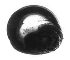
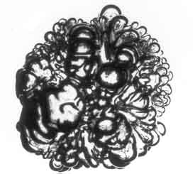
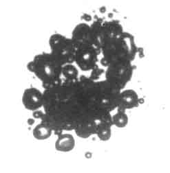
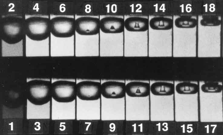
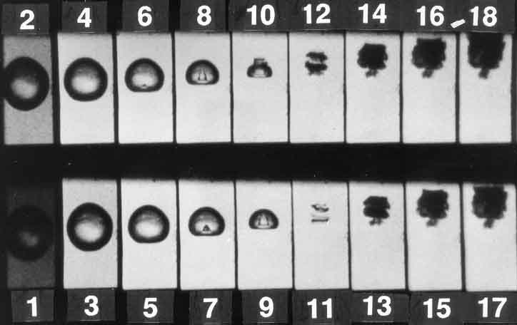
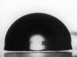
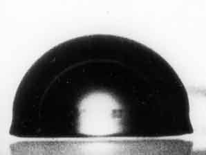
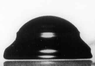
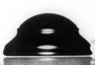
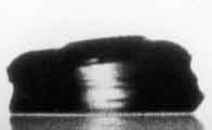
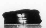
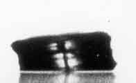
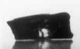
On the the hand, it is clear from the theory that the bubble may become highly unstable to nonspherical disturbances during stage two because d²R/dt² reaches very large positive values during this rebound phase. The instability appears to manifest itself in several different ways depending on the violence of the collapse and the presence of other boundaries. All vapor bubbles that collapse to a size orders of magnitude smaller than their maximum size inevitably emerge from that collapse as a cloud of smaller bubbles rather than a single vapor bubble. This fragmentation could be caused by a single microjet as described below, or it could be due to a spherical harmonic disturbance of higher order. The behavior of collapsing bubbles that are predominantly gas filled (or bubbles whose collapse is thermally inhibited) is less certain since the lower values of d²R/dt² in those cases make the instability weaker and, in some cases, could imply spherical stability. Thus acoustically excited cavitation bubbles that contain substantial gas often remain spherical during their rebound phase. In other instances the instability is sufficient to cause fragmentation. Several examples of fragmented and highly distorted bubbles emerging from the rebound phase are shown in Figure 3.3. These are from the experiments of Frost and Sturtevant (1986), in which the thermal effects are substantial.

Figure 3.3 Photographs of an ether bubble in glycerine before (left) and after (center) a collapse and rebound. The cloud on the right is the result of a succession of collapse and rebound cycles. Reproduced from Frost and Sturtevant (1986) with the permission of the authors.

Figure 3.4 Photograph of a collapsing bubble showing the initial development of the reentrant microjet caused by a solid but transparent wall whose location is marked by the dotted line. From Benjamin and Ellis (1966) reproduced with permission of the first author.

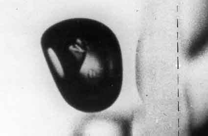
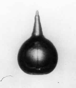
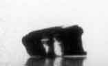
A dominant feature in the collapse of many vapor bubbles is the development of a reentrant jet (the n=2 mode) due to an asymmetry such as the presence of a nearby solid boundary. Such an asymmetry causes one side of the bubble to accelerate inward more rapidly than the opposite side and this results in the development of a high-speed re-entrant microjet which penetrates the bubble. Such microjets were first observed experimentally by Naude and Ellis (1961) and Benjamin and Ellis (1966). Of particular interest for cavitation damage is the fact that a nearby solid boundary will cause a microjet directed toward that boundary. Figure 3.4, from Benjamin and Ellis (1966), shows the initial formation of the microjet directed at a nearby wall. Other asymmetries, even gravity, can cause the formation of these reentrant microjets. Figure 3.5 is one of the very first, if not the first, photographs taken showing the result of a gravity-produced upward jet having progressed through the bubble and penetrated into the fluid on the other side thus creating the spiky protuberance. Indeed, the upward inclination of the wall-induced reentrant jet in Figure 3.4 is caused by gravity. Figure 3.6 presents a comparison between the reentrant jet development in a bubble collapsing near a solid wall as observed by Lauterborn and Bolle (1975) and as computed by Plesset and Chapman (1971).

Figure 3.5 Photograph from Benjamin and Ellis (1966) showing the protuberence generated when a gravity-induced upward-directed reentrant jet progresses through the bubble and penetrates the fluid on the other side. Reproduced with permission of the first author.

Figure 3.6 The collapse of a cavitation bubble close to a solid boundary in a quiescent liquid. The theoretical shapes of Plesset and Chapman (1971) (solid lines) are compared with the experimental observations of Lauterborn and Bolle (1975) (points). Figure adapted from Plesset and Prosperetti (1977).

Another asymmetry that can cause the formation of a reentrant jet is the proximity of other, neighboring bubbles in a finite cloud of bubbles. Then, as Chahine and Duraiswami (1992) have shown in their numerical calculations, the bubbles on the outer edge of such a cloud will tend to develop jets directed toward the center of the cloud; an example is shown in Figure 3.7. Other manifestations include a bubble collapsing near a free surface, that produces a reentrant jet directed away from the free surface (Chahine 1977). Indeed, there exists a critical surface flexibility separating the circumstances in which the reentrant jet is directed away from rather than toward the surface. Gibson and Blake (1982) demonstrated this experimentally and analytically and suggested flexible coatings or liners as a means of avoiding cavitation damage. It might also be noted that depth charges rely for their destructive power on a reentrant jet directed toward the submarine upon the collapse of the explosively generated bubble.

Figure 3.7 Numerical calculation of the collapse of a group of five bubbles showing the development of inward-directed reentrant jets on the outer four bubbles. From Chahine and Duraiswami (1992) reproduced with permission of the authors.

Many other experimentalists have subsequently observed reentrant jets (or ``microjets'') in the collapse of cavitation bubbles near solid walls. The progress of events seems to differ somewhat depending on the initial distance of the bubble center from the wall. When the bubble is initially spherical but close to the wall, the typical development of the microjet is as illustrated in Figure 3.8, a series of photographs taken by Tomita and Shima (1990). When the bubble is further away from the wall, the later events are somewhat different; another set of photographs taken by Tomita and Shima (1990) is included as Figure 3.9 and shows the formation of two toroidal vortex bubbles (frame 11) after the microjet has completed its penetration of the original bubble. Furthermore, the photographs of Lauterborn and Bolle (1975) in which the bubbles are about a diameter from the wall, show that the initial collapse is quite spherical and that the reentrant jet penetrates the fluid between the bubble and the wall as the bubble is rebounding from the first collapse. At this stage the appearance is very similar to Figure 3.5 but with the protuberance directed at the wall.

Figure 3.8 Series of photographs showing the development of the microjet in a bubble collapsing very close to a solid wall (at top of frame). The interval between the numbered frames is 2μs and the frame width is 1.4mm. From Tomita and Shima (1990), reproduced with permission of the authors.

Figure 3.9 A series of photographs similar to the previous figure but with a larger separation from the wall. From Tomita and Shima (1990), reproduced with permission of the authors.

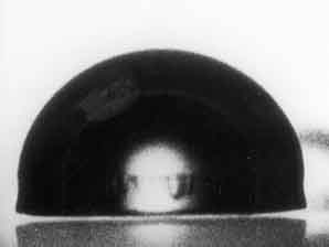
Figure 3.10 Series of photographs of a hemispherical bubble collapsing against a wall showing the ``pancaking'' mode of collapse. Four groups of three closely spaced photographs beginning at top left and ending at the bottom right. From Benjamin and Ellis (1966) reproduced with permission of the first author.

On the other hand, when the initial bubble is much closer to the wall and collapse begins from a spherical cap shape, the photographs (for example, Shima et al. (1981) or Kimoto (1987)) show a bubble that ``pancakes'' down toward the surface in a manner illustrated by Figure 3.10 taken from Benjamin and Ellis (1966). In these circumstances it is difficult to observe the microjet.

The reentrant jet phenomenon in a quiescent fluid has been extensively studied analytically as well as experimentally. Plesset and Chapman (1971) numerically calculated the distortion of an initially spherical bubble as it collapsed close to a solid boundary and, as Figure 3.6, their profiles are in good agreement with the experimental observations of Lauterborn and Bolle (1975). Blake and Gibson (1987) review the current state of knowledge, particularly the analytical methods for solving for bubbles collapsing near a solid or a flexible surface.

When a bubble in a quiescent fluid collapses near a wall, the reentrant jets reach high speeds quite early in the collapse process and long before the volume reaches a size at which, for example, liquid compressibility becomes important (see Section 3.2). The speed of the reentrant jet, U_J, at the time it impacts the opposite surface of the bubble has been shown to be given by

	......(3.9)

where ξ is a constant and Δp is the difference between the remote pressure, which would maintain the bubble at equilibrium at its maximum or initial radius, and the remote pressure present during collapse. Gibson (1968) found that ξ=7.6 fit his experimental observations; Blake and Gibson (1987) indicate that ξ is a function of the ratio, C, of the initial distance of the bubble center from the wall to the initial radius and that ξ=11.0 for C=1.5 and ξ=8.6 for C=1.0. Voinov and Voinov (1975) found that the value of ξ could be as high as 64 if the initial bubble had a slightly eccentric shape.

Whether the bubble is fissioned due to the disruption caused by the microjet or by the effects of the stage two instability, many of the experimental observations of bubble collapse (for example, those of Kimoto 1987) show that a bubble emerges from the first rebound not as a single bubble but as a cloud of smaller bubbles. Unfortunately, the events of the last moments of collapse occur so rapidly that the experiments do not have the temporal resolution neccessary to show the details of this fission process. The subsequent dynamical behavior of the bubble cloud may be different from that of a single bubble. For example, the damping of the rebound and collapse cycles is greater than for a single bubble.

Finally, it is important to emphasize that virtually all of the observations described above pertain to bubble collapse in an otherwise quiescent fluid. A bubble that grows and collapses in a flow is subject to other deformations that can significantly alter the noise and damage potential of the collapse process. In Chapter 7 this issue will be addressed further.

 

3.6 CAVITATION DAMAGE

Perhaps the most ubiqitous engineering problem caused by cavitation is the material damage that cavitation bubbles can cause when they collapse in the vicinity of a solid surface. Consequently, this subject has been studied quite intensively for many years (see, for example, ASTM 1967; Thiruvengadam 1967, 1974; Knapp, Daily, and Hammitt 1970). The problem is a difficult one because it involves complicated unsteady flow phenomena combined with the reaction of the particular material of which the solid surface is made. Though there exist many empirical rules designed to help the engineer evaluate the potential cavitation damage rate in a given application, there remain a number of basic questions regarding the fundamental mechanisms involved.

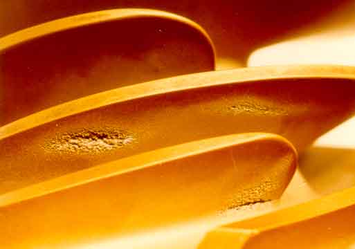
In the preceding sections, we have seen that cavitation bubble collapse is a violent process that generates highly localized, large-amplitude shock waves (Section 3.2) and microjets (Section 3.5) in the fluid at the point of collapse. When this collapse occurs close to a solid surface, these intense disturbances generate highly localized and transient surface stresses. Repetition of this loading due to repeated collapses causes local surface fatigue failure and the subsequent detachment or flaking off of pieces of material. This is the generally accepted explanation of cavitation damage. It is also consistent with the metallurgical evidence of damage in harder materials. Figure 3.11 is a typical photograph of localized cavitation damage on a pump blade. It usually has the jagged, crystalline appearance consistent with fatigue failure and is usually fairly easy to distinguish from the erosion due to solid particles, which has a much smoother appearance. With iron or steel, the effects of corrosion often enhance the speed of cavitation damage.

Figure 3.11 Photograph of typical cavitation damage on the blade of a mixed flow pump.

Parenthetically it should be noted that pits caused by individual bubble collapses are often observed with soft materials, and the relative ease with which this process can be studied experimentally has led to a substantial body of research evidence for soft materials. Much of this literature implies that the microjets cause the individual pits. However, it does not neccessarily follow that the same mechanism causes the damage in harder materials.

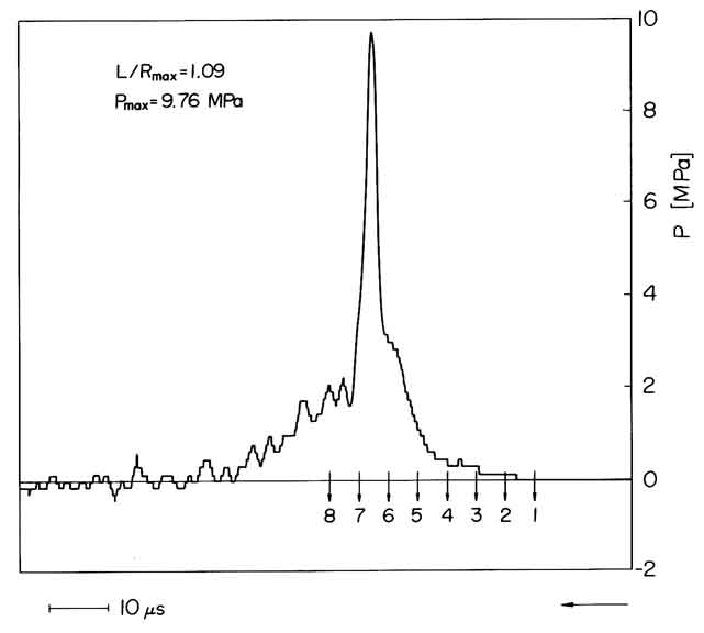
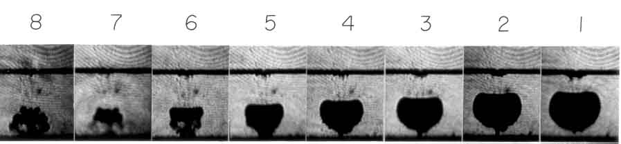
Indeed, the issue of whether cavitation damage is caused by microjets or by shock waves or by both has been debated for many years. In the 1940s and 1950s the focus was on the shock waves generated by spherical bubble collapse. When the phenomenon of the microjet was first observed by Naude and Ellis (1961) and Benjamin and Ellis (1966), the focus shifted to studies of the impulsive pressures generated by these jets. But, even after the disruption caused by the microjet, one is left with a remnant cloud of small bubbles that will continue to collapse collectively. Though no longer a single bubble, this remnant cloud will still exhibit the same qualitative dynamic behavior, including the possible production of a shock wave following the point of minimum cavity volume. Two important research efforts in Japan then shifted the focus back to the remnant cloud shock. First Shima et al. (1983) used high speed Schlieren photography to show that a spherical shock wave was indeed generated by the remnant cloud at the instance of minimum volume. Figure 3.12 shows a series of photographs of a collapsing bubble along with the corresponding pressure trace. The instant of minimum volume is between frames 6 and 7, and the trace clearly shows the peak pressure occuring at that instant. When combined with the Schlieren photographs showing a spherical shock being generated at this instant, this seemed to relegate the microjet to a subsidiary role. About the same time, Fujikawa and Akamatsu (1980) used a photoelastic material so that they could simultaneously observe the stresses in the solid and measure the acoustic pulses. Using the first collapse of a bubble as the trigger, Fujikawa and Akamatsu employed a variable time delay to take photographs of the stress state in the solid at various instants relative to the second collapse. They simultaneously recorded the pressure in the liquid and were able to confirm that the impulsive stresses in the material were initiated at the same moment as the acoustic pulse (to within about 1μs). They also conclude that this corresponded to the instant of minimum volume and that the waves were not produced by the microjet.

Figure 3.12 Series of photographs of a cavitation bubble collapsing near a wall along with the characteristic wall pressure trace. The time corresponding to each photograph is marked by a number on the trace. From Shima, Takayama, Tomita, and Ohsawa (1983) reproduced with permission of the authors.

However, in a later investigation, Kimoto (1987) was able to observe stress pulses that resulted both from microjet impingement and from the remnant cloud collapse shock. Typically, the impulsive pressures from the latter are 2 to 3 times larger than those due to the microjet, but it would seem that both may contribute to the impulsive loading of the surface.

For detailed experimental evaluation of the comparative susceptibility of various materials to cavitation damage, the reader is referred to Knapp, Daily, and Hammitt (1970). Standard devices have been been used to evaluate these comparative susceptibilities. The most common consists of a device that oscillates a specimen in a liquid, producing periodic growth and collapse of cavitation bubbles on the face of the specimen. The tests are conducted over many hours with regular weighing to determine the weight loss. It transpires that the rate of loss of material is not constant. Causes suggested for changes in the rate of loss of material include time constants associated with the fatigue process and the fact that an irregular, damaged surface may produce an altered pattern of cavitation. Commonly, these test cells are operated by a magnetostrictive device in order to achieve the standard frequencies of 5kHz or, sometimes, 20kHz. These frequencies cause the largest cavitating bubble clouds on the surface of the specimen because they are close to the natural frequencies of a significant fraction of the nuclei present in the liquid (see Section 4.2). In addition to the magnetostrictive devices, standard material susceptibility tests are also carried out using cavitating venturis and rotating disks.

In most practical devices, cavitation damage is a very undesirable. However, there are some circumstances in which the phenomenon is used to advantage. It is believed, for example, that the mechanics of rock-cutting by high speed water jets is caused, at least in part, by cavitation in the jet as it flows over a rough rock surface. Many readers have also been subjected to the teeth-cleaning power of the small, high-speed cavitating water jets used by dentists; those with dentures may also have successfully employed acoustic cavitation to clean their dentures in commercial acoustic cleaners. On the other side of the coin, the violence of a collapsing bubble is suspected of causing major tissue damage in head injuries.

 

3.7 DAMAGE DUE TO CLOUD COLLAPSE

Figure 3.13 Photograph of a transient cloud of cavitation bubbles generated acoustically. From Plesset and Ellis (1955).

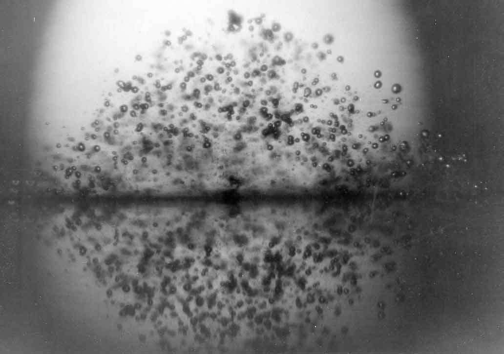
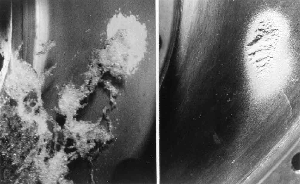
In many practical devices cavitation damage is observed to occur in quite localized areas, for example, in a pump impeller. Often this is the result of the periodic and coherent collapse of a cloud of cavitation bubbles. Such is the case in the magnetostrictive cavitation testing equipment mentioned above. A typical cloud of bubbles generated by such acoustic means is shown in Figure 3.13. In other hydraulic machines, the periodicity may occur naturally as a result of regular shedding of cavitating vortices, or it may be a response to a periodic disturbance imposed on the flow. Example of the kinds of imposed fluctuations are the interaction between a row of rotor vanes and a row of stator vanes in a pump or turbine or the interaction between a ship's propeller and the nonuniform wake behind the ship. In almost all such cases the coherent collapse of the cloud can cause much more intense noise and more potential for damage than in a similar nonfluctuating flow. Consequently the damage is most severe on the solid surface close to the location of cloud collapse. An example of this phenomenon is included in Figure 3.14 taken from Soyama, Kato, and Oba (1992). In this instance clouds of cavitation are being shed from the leading edge of a centrifugal pump blade and are collapsing in a specific location, as suggested by the pattern of cavitation in the left-hand photograph. This leads to the localized damage shown in the right-hand photograph.

Figure 3.14 Axial views from the inlet of the cavitation and cavitation damage on the hub or base plate of a centrifugal pump impeller. The two photographs are of the same area, the one on the left showing the typical cavitation pattern during flow and the one on the right the typical cavitation damage. Parts of the blades can be seen in the upper left and lower right corners. Relative to these blades, the flow proceeds from the lower left to the upper right. The leading edge of the blade in upper left is just outside the field of view on the left. Reproduced from Soyama, Kato, and Oba (1992) with permission of the authors.

At the time of writing, a number of research efforts are focusing on the dynamics of cavitation clouds. Later, in Section 6.10, we analyze some of the basic dynamics of spherical bubble clouds and show that the interaction between bubbles lead to a coherent dynamics of the cloud, including natural frequencies that can be much smaller than the natural frequencies of individual bubbles. These studies suggest that the coherent collapse can be more violent than that of individual bubbles. However, a complete explanation for the increase in the noise and damage potential does not yet exist.

 

3.8 CAVITATION NOISE

The violent and catastrophic collapse of cavitation bubbles results in the production of noise as well as the possibility of material damage to nearby solid surfaces. The noise is a consequence of the momentary large pressures that are generated when the contents of the bubble are highly compressed. Consider the flow in the liquid caused by the volume displacement of a growing or collapsing cavity. In the far field the flow will approach that of a simple source, and it is clear that Equation 2.7 for the pressure will be dominated by the first term on the right-hand side (the unsteady inertial term) since it decays more slowly with radius, r, than the second term. If we denote the time-varying volume of the cavity by V(t) and substitute using Equation 2.2, it follows that the time-varying component of the pressure in the far field is given by

	......(3.10)

where p_a is the radiated acoustic pressure and we denote the distance, r, from the cavity center to the point of measurement by (for a more thorough treatment see Dowling and Ffowcs Williams 1983 and Blake 1986b). Since the noise is directly proportional to the second derivative of the volume with respect to time, it is clear that the noise pulse generated at bubble collapse occurs because of the very large and positive values of d²V/dt² when the bubble is close to its minimum size. It is conventional (see, for example, Blake 1986b) to present the sound level using a root mean square pressure or acoustic pressure, p_s, defined by

	......(3.11)

and to represent the distribution over the frequency range, f, by the spectral density function, (f).

The crackling noise that accompanies cavitation is one of the most evident characteristics of this phenomenon to the researcher or engineer. The onset of cavitation is often detected first by this noise rather than by visual observation of the bubbles. Moreover, for the practical engineer it is often the primary means of detecting cavitation in devices such as pumps and valves. Indeed, several empirical methods have been suggested that estimate the rate of material damage by measuring the noise generated (for example, Lush and Angell 1984).

The noise due to cavitation in the orifice of a hydraulic control valve is typical, and spectra from such an experiment are presented in Figure 3.15. The lowest curve at σ=0.523 represents the turbulent noise from the noncavitating flow. Below the incipient cavitation number (about 0.523 in this case) there is a dramatic increase in the noise level at frequencies of about 5kHz and above. The spectral peak between 5kHz and 10kHz corresponds closely to the expected natural frequencies of the nuclei present in the flow (see Section 4.2).

Figure 3.15 Acoustic power spectra from a model spool valve operating under noncavitating (σ=0.523) and cavitating (σ=0.452 and 0.342) conditions (from the investigation of Martin et al. 1981).

Most of the analytical approaches to cavitation noise build on knowledge of the dynamics of collapse of a single bubble. Fourier analyses of the radiated acoustic pressure due to a single bubble were first visualized by Rayleigh (1917) and implemented by Mellen (1954) and Fitzpatrick and Strasberg (1956). In considering such Fourier analyses, it is convenient to nondimensionalize the frequency by the typical time span of the whole event or, equivalently, by the collapse time, t_TC, given by Equation 2.40. Now consider the frequency content of (f) using the dimensionless frequency, ft_TC. Since the volume of the bubble increases from zero to a finite value and then returns to zero, it follows that for ft_TC<1 the Fourier transform of the volume is independent of frequency. Consequently d²V/dt² will be proportional to f ² and therefore (f) is proportional to f ⁴ (see Fitzpatrick and Strasberg 1956). This is the origin of the left-hand asymptote in Figure 3.16. The behavior at intermediate frequencies for which ft_TC>1 has been the subject of more speculation and debate. Mellen (1954) and others considered the typical equations governing the collapse of a spherical bubble in the absence of thermal effects and noncondensable gas (Equation 2.36) and concluded that, since the velocity dR/dt is proportional to R^-3/2, it follows that R behaves like t^2/5. Therefore the Fourier transform of d²V/dt² leads to an asymptotic behavior in which (f) is proportional to f ^-2/5. The error in this analysis is the neglect of the noncondensable gas. When this is included and when the collapse is sufficiently advanced, the last term in the square brackets of Equation 2.36 becomes comparable with the previous terms. Then the evolution of is quite different from t^2/5. Moreover, the values of d²V/dt² are much larger during this rebound phase, and therefore the frequency content of the rebound phase will dominate the spectrum. It is therefore not surprising that the f ^-2/5 is not observed in practice. Rather, most of the experimental results seem to exhibit an intermediate frequency behavior like f ^-1 or f ^-2. Jorgensen (1961) measured the noise from submerged, cavitating jets and found a behavior like f ^-2 at the higher frequencies (see Figure 3.16). However, most of the experimental data for cavitating bodies or hydrofoils exhibit a weaker decay. The data by Arakeri and Shangumanathan (1985) from cavitating headform experiments show a very consistent f ^-1 trend over almost the entire frequency range, and very similar results have been obtained by Ceccio and Brennen (1991) (see Figure 3.20). Though the data of Blake et al. (1977) for a cavitating hydrofoil exhibit some consistent peaks, the overall trend in their data is also consistent with f ^-1. This is also the asymptotic behavior exhibited at higher frequencies by the data of Barker (1973) for a cavitating foil.

Several authors have also analyzed the effects of the compressibility of the liquid. Mellen (1954) and Fitzpatrick and Strasberg (1956) conclude that this causes faster decay like f ^-2 above some critical frequency, though this has not been clearly demonstrated experimentally. In Figure 3.16 typical functional behaviors of (f) have been included in a graph showing measurements of some of the noise from a cavitating jet taken by Jorgensen (1961).

Figure 3.16 Acoustic power spectra of the noise from a cavitating jet. Shown are mean lines through two sets of data constructed by Blake and Sevik (1982) from the data by Jorgensen (1961). Typical asymptotic behaviors are also indicated. The reference frequency, fR, is (p∞/ρLD2)½ where D is the jet diameter.

The peaks in many of the spectra of the noise from cavitating flows (for example those of Figures 3.15 and 3.16) tend to lower frequencies as the cavitation number decreases, primarily because of an increase in the amplitude of the higher frequencies. This trend is further illustrated by the data for cavitating jets presented in Figure 3.17. Given some form for the asymptotes at high and low frequency and some functional behavior for the location of the peak frequency, it is not unreasonable to seek to reduce the measured spectra for a given type of cavitating flow to some universal form. Arakeri and Shangumanathan (1985) were able to reduce the noise spectra from cavitating headform experiments to a single band provided the bubble population was low enough to eliminate bubble/bubble interaction. Blake (1986a) has attempted a similar task for the various kinds of cavitation that can occur on a propeller, since the ability to scale from model tests to the prototype is important in that context. There remain, however, a number of unresolved issues that seem to demand a closer examination of the basic mechanics of noise production even in the absence of bubble/bubble interactions.

Figure 3.17 Frequency of the peak in the acoustic spectra as a function of cavitation number. Data for cavitating jets from Franklin and McMillan (1984). The jet diameter and mean velocity are denoted by D and u.

Recently Ceccio and Brennen (1991) have recorded the noise from individual cavitation bubbles in a flow; a typical acoustic signal from their experiments is reproduced in Figure 3.18. The large positive pulse at about 450μs corresponds to the first collapse of the bubble. This first pulse in Figure 3.18 is followed by some facility-dependent oscillations and by a second pulse at about 1100μs . This corresponds to the second collapse, which follows the rebound from the first collapse. Further rebounds are possible but were not observed in these experiments.

Figure 3.18 A typical acoustic signal from a single collapsing bubble. From Ceccio and Brennen (1991).

Figure 3.19 Comparison of the acoustic impulse, I, produced by the collapse of a single cavitation bubble on two axisymmetric headforms as a function of the maximum volume prior to collapse. Open symbols: average data for Schiebe headform; closed symbols: ITTC headform; vertical lines indicate one standard deviation. Also shown are the corresponding results from the solution of the Rayleigh-Plesset equation. From Ceccio and Brennen (1991).

A good measure of the magnitude of the collapse pulse is the acoustic impulse, I, defined as the area under the pulse or

	......(3.12)

where t₁ and t₂ are times before and after the pulse at which p_a is zero. For later purposes we also define a dimensionless impulse, I^*, as

	......(3.13)

where U_∞ and R_H are the reference velocity and length in the flow. The average acoustic impulses for individual bubble collapses on two axisymmetric headforms (ITTC and Schiebe headforms) are compared in Figure 3.19 with impulses predicted from integration of the Rayleigh-Plesset equation. Since these theoretical calculations assume that the bubble remains spherical, the discrepancy between the theory and the experiments is not too surprising. Indeed one interpretation of Figure 3.19 is that the theory can provide an order of magnitude estimate and an upper bound on the noise produced by a single bubble. In actuality, the departure from sphericity produces a less focused collapse and therefore less noise.

Typical spectra showing the frequency content in single bubble noise are included in Figure 3.20. If the events are randomly distributed in time (see below), this would also correspond to the overall cavitation noise spectrum. These spectra exhibit the previously mentioned f ^-1 behavior for the range 1→50kHz; the rapid decline at about 80kHz represents the limit of the hydrophone used to make these measurements.

Figure 3.20 Typical spectra of noise from bubble cavitation for various cavitation numbers. From Ceccio and Brennen (1991).

The next step is to consider the synthesis of cavitation noise from the noise produced by individual cavitation bubbles or events. This is a fairly simple matter provided the events can be considered to occur randomly in time. At low nuclei population densities the evidence suggests that this is indeed the case (see, for example, Morozov 1969). Baiter, Gruneis, and Tilmann (1982) have explored the consequences of the departures from randomness that could occur at larger bubble population densities. Here, we limit the analysis to the case of random events. Then, if the impulse produced by each event is denoted by I and the number of events per unit time is denoted by , the sound pressure level, p_s, will be given by

	......(3.14)

Consider the scaling of cavitation noise that is implicit in this construct. We shall omit some factors of proportionality for the sake of clarity, so the results are only intended as a qualitative guide.

Both the experimental results and the analysis based on the Rayleigh-Plesset equation indicate that the nondimensional impulse produced by a single cavitation event is strongly correlated with the maximum volume of the bubble prior to collapse and is almost independent of the other flow parameters. It follows from Equations 3.10 and 3.12 that

	......(3.15)

and the values of dV/dt at the moments t=t₁, t₂ when d²V/dt²=0 may be obtained from the Rayleigh-Plesset equation. If the bubble radius at the time t₁ is denoted by R_X and the coefficient of pressure in the liquid at that moment is denoted by C_px, then

	......(3.16)

Numerical integrations of the Rayleigh-Plesset equation for a range of typical circumstances indicate that R_X/R_M is approximately 0.62 where R_M is the maximum volumetric radius and that (C_px-σ) is proportional to R_M/R_H so that

	......(3.17)

The aforementioned integrations of the Rayleigh-Plesset equation yield a factor of proportionality, β, of about 35. Moreover, the upper envelope of the experimental data of which Figure 3.19 is a sample appears to correspond to a value of β of approximately 4. We note that a quite similar relation between I^* and R_M/R_H emerges from the analysis by Esipov and Naugol'nykh (1973) of the compressive sound wave generated by the collapse of a gas bubble in a compressible liquid. Indeed, the compressibility of the liquid does not appear to affect the acoustic impulse significantly.

From the above relations, it follows that

	......(3.18)

Consequently, the evaluation of the impulse from a single event is completed by some estimate of R_M. Previously (Section 2.5) we evaluated R_M and showed it to be independent of U_∞ for a given cavitation number. In that case I is linear with U_∞.

The event rate, , can be considerably more complicated to evaluate than might at first be thought. If all the nuclei flowing through a certain, known streamtube (say with a cross-sectional area in the upstream flow of A_N) were to cavitate similarly, then the result would be

	......(3.19)

where N is the nuclei concentration (number/unit volume) in the incoming flow. Then it follows that the acoustic pressure level resulting from substituting Equations 3.19, 3.18 and 2.52 into Equation 3.14 becomes

	......(3.20)

where we have omitted some of the constants of order unity. For the relatively simple flows considered here, Equation 3.20 yields a sound pressure level that scales with U_∞² and with R_H⁴ because A_N is proportional to R_H². This scaling with velocity does correspond roughly to that which has been observed in some experiments on traveling bubble cavitation, for example, those of Blake, Wolpert, and Geib (1977) and Arakeri and Shangumanathan (1985). The former observe that p_s is proportional to U_∞^m where m=1.5 to 2. There are, however, a number of complicating factors that can alter these scaling relationships. First, as we have discussed earlier in Section 2.5, only those nuclei larger than a certain critical size, R_c, will actually grow to become cavitation bubbles. Since R_c is a function of both σ and the velocity, U_∞, this means that the effective N will be a function of R_c and U_∞. Since R_c decreases as U_∞ increases, this would tend to produce powers, m, somewhat greater than 2. But it is also the case that, in any experimental facility, N will typically change with U_∞ in some facility-dependent manner. Often this will cause N to decrease with U_∞ at constant σ (since N will typically decrease with increasing tunnel pressure), and this effect would then produce values of m that are less than 2.

Different scaling laws will apply when the cavitation is generated by turbulent fluctuations such as in a turbulent jet (see, for example, Ooi 1985 and Franklin and McMillan 1984). Then the typical tension experienced by a nucleus as it moves along a disturbed path in a turbulent flow is very much more difficult to estimate. Consequently, the models for the sound pressure due to cavitation and the scaling of that sound with velocity are less well understood.

When the population of bubbles becomes sufficiently large, the radiated noise will begin to be affected by the interactions between the bubbles. In Chapters 6 and 7 we discuss some analyses and some of the consequences of these interactions in clouds of cavitating bubbles. There are also a number of experimental studies of the noise from the collapse of cavitating clouds, for example, that of Bark and van Berlekom (1978).

 

3.9 CAVITATION LUMINESCENCE

Though highly localized both temporally and spatially, the extremely high temperatures and pressures that can occur in the noncondensable gas during collapse are believed to be responsible for the phenomenon known as luminescence, the emission of light that is observed during cavitation bubble collapse. The phenomenon was first observed by Marinesco and Trillat (1933), and a number of different explanations were advanced to explain the emissions. The fact that the light was being emitted at collapse was first demonstrated by Meyer and Kuttruff (1959). They observed cavitation on the face of a rod oscillating magnetostrictively and correlated the light with the collapse point in the growth-and-collapse cycle. The balance of evidence now seems to confirm the suggestion by Noltingk and Neppiras (1950) that the phenomenon is caused by the compression and adiabatic heating of the noncondensable gas in the collapsing bubble. As we discussed previously in Sections 2.4 and 3.4, temperatures of the order of 6000°K can be anticipated on the basis of uniform compression of the noncondensable gas; the same calculations suggest that these high temperatures will last for only a fraction of a microsecond. Such conditions would indeed explain the emission of light. Indeed, the measurements of the spectrum of sonoluminescence by Taylor and Jarman (1970), Flint and Suslick (1991), and others suggest a temperature of about 5000°K. However, some recent experiments by Barber and Putterman (1991) indicate much higher temperatures and even shorter emission durations of the order of picoseconds. Speculations on the explanation for these observations have centered on the suggestion by Jarman (1960) that the collapsing bubble forms a spherical, inward-propagating shock in the gas contents of the bubble and that the focusing of the shock at the center of the bubble is an important reason for the extremely high apparent ``temperatures'' associated with the sonoluminescence radiation. It is, however, important to observe that spherical symmetry is essential for this mechanism to have any significant consequences. One would therefore expect that the distortions caused by a flow would not allow significant shock focusing and would even reduce the effectiveness of the basic compression mechanism.

When it occurs in the context of acoustic cavitation (see Chapter 4), luminescence is called sonoluminescence despite the evidence that it is the cavitation rather than the sound that causes the light emission. Sonoluminescence and the associated chemistry that is induced by the high temperatures and pressures (known as ``sonochemistry'') have been more thoroughly investigated than the corresponding processes in hydrodynamic cavitation. However, the subject is beyond the scope of this book and the reader is referred to other works such as the book by Young (1989).

As one would expect from the Rayleigh-Plesset equation, the surface tension and vapor pressure of the liquid are important in determining the sonoluminescence flux as the data of Jarman (1959) clearly show (see Figure 3.21). Certain aqueous solutes like sodium disulphide seem to enhance the luminescence, though it is not clear that the same mechanism is responsible for the light emission under these circumstances. Sonoluminescence is also strongly dependent on the thermal conductivity of the gas (Hickling 1963, Young 1976), and this is particularly evident with gases like xenon and krypton, which have low thermal conductivities. Clearly then, the conduction of heat in the gas plays an important role in the phenomenon. Therefore, the breakup of the bubble prior to complete collapse might be expected to eliminate the phenomenon completely.

Figure 3.21 The correlation of the sonoluminescence flux with S2/pV for data in a variety of liquids. From Jarman (1959).

Light emission in a cavitating flow was first investigated by Jarman and Taylor (1964, 1965) who observed luminescence in a cavitating venturi and identified the source as the region of bubble collapse. They also found that an acoustic pressure pulse was associated with each flash of light. The maximum emission was in a band of wavelengths around 5000 angstroms, which is in accord with the many apocryphal accounts of steady or flashing blue light emanating from flowing water. Peterson and Anderson (1967) also conducted experiments with venturis and explored the effects of different, noncondensable gases dissolved in the water. They observe that the emission of light implies blackbody sources with a temperature above 6000°K. There are, however, other experimenters who found it very difficult to observe any luminescence in a cavitating flow. One suspects that only bubbles that collapse with significant spherical symmetry will actually produce luminescence. Such events may be exceedingly rare in many flows.

The phenomenon of luminescence is not just of academic interest. For one thing there is evidence that it may initiate explosions in liquid explosives (Gordeev et al. 1967). More constructively, there seems to be significant interest in utilizing the chemical-processing potential of the high temperatures and pressures in what is otherwise a benign environment. For example, it is possible to use cavitation to break up harmful molecules in water (Dahi 1982).

REFERENCES

• ASTM. (1967). Erosion by cavitation or impingement. Amer. Soc. for Testing and Materials, ASTM STP408.
• Akulichev, V.A. (1971). High intensity ultrasonic fields. L.D. Rosenberg (ed.), Plenum Press.
• Arakeri, V.H. and Shangumanathan, V. (1985). On the evidence for the effect of bubble interference on cavitation noise. J. Fluid Mech., 159, 131--150.
• Baiter, H.-J., Gruneis, F. and Tilmann, P. (1982). An extended base for the statistical description of cavitation noise. Proc. ASME Int. Symp. on Cavitation Noise, 93--108.
• Barber, B.P. and Putterman, S.J. (1991). Observations of synchronous picosecond sonluminescence. Nature, 352, 318.
• Bark, G. and van Berlekom, W.B. (1978). Experimental investigations of cavitation noise. Proc. 12th ONR Symp. on Naval Hydrodynamics, 470--493.
• Barker, S.J. (1973). Measurements of radiated noise from cavitating hydrofoils. ASME Cavitation and Polyphase Flow Forum, 27--30.
• Benjamin, T.B. (1958). Pressure waves from collapsing cavities. Proc. Second ONR Symp. Naval Hyrodynamics, 207--233.
• Benjamin, T.B. and Ellis, A.T. (1966). The collapse of cavitation bubbles and the pressures thereby produced against solid boundaries. Phil. Trans. Roy. Soc., London, Ser. A, 260, 221--240.
• Blake, J.R. and Gibson, D.C. (1987). Cavitation bubbles near boundaries. Ann. Rev. Fluid Mech., 19, 99--124.
• Blake, W.K., Wolpert, M.J. and Geib, F.E. (1977). Cavitation noise and inception as influenced by boundary-layer development on a hydrofoil. J. Fluid Mech., 80, 617--640.
• Blake, W.K. and Sevik, M.M. (1982). Recent developments in cavitation noise research. Proc. ASME Int. Symp. on Cavitation Noise, 1--10.
• Blake, W.K. (1986a). Propeller cavitation noise: the problems of scaling and prediction. Proc. ASME Int. Symp. on Cavitation Noise, 89--99.
• Blake, W.K. (1986b). Mechanics of flow-induced sound and vibration. Academic Press.
• Ceccio, S.L. and Brennen, C.E. (1991). Observations of the dynamics and acoustics of travelling bubble cavitation. J. Fluid Mech., 233, 633--660.
• Chahine, G.L. (1977). Interaction between an oscillating bubble and a free surface. ASME J. Fluids Eng., 99, 709--716.
• Chahine, G.L. and Duraiswami, R. (1992). Dynamical interactions in a multibubble cloud. ASME J. Fluids Eng., 114, 680--686.
• Dahi, E. (1982). Perspective of combination of ozone and ultrasound. In Ozonization Manual for Water and Wastewater Treatment (editor W.J.Masschelein), John Wiley and Sons.
• Dowling, A.P. and Ffowcs Williams, J.E. (1983). Sound and sources of sound. Ellis Horwood Ltd. and John Wiley and Sons.
• Esipov, I.B. and Naugol'nykh, K.A. (1973). Collapse of a bubble in a compressible liquid. Akust. Zh., 19, 285--288.
• Fitzpatrick, H.M. and Strasberg, M. (1956). Hydrodynamic sources of sound. Proc. First ONR Symp. on Naval Hydrodynamics, 241--280.
• Flint, E.B. and Suslick, K.S. (1991). The temperature of cavitation. Science, 253, 1397--1399.
• Flynn, H.G. (1966). Cavitation dynamics. I, A mathematical formulation. Acoust. Res. Lab., Harvard Univ., Tech. Memo. 50.
• Franklin, R.E. and McMillan, J. (1984). Noise generation in cavitating flows, the submerged jet. ASME J. Fluids Eng., 106, 336--341.
• Frost, D. and Sturtevant, B. (1986). Effects of ambient pressure on the instability of a liquid boiling explosively at the superheat limit. ASME J. Heat Transfer, 108, 418--424.
• Fujikawa, S. and Akamatsu, T. (1980). Effects of the non-equilibrium condensation of vapour on the pressure wave produced by the collapse of a bubble in a liquid. J. Fluid Mech., 97, 481--512.
• Gibson, D.C. (1968). Cavitation adjacent to plane boundaries. Proc. Australian Conf. on Hydraulics and Fluid Machinery, 210--214.
• Gibson, D.C. and Blake, J.R. (1982). The growth and collapse of bubbles near deformable surfaces. Appl. Sci. Res., 38, 215--224.
• Gilmore, F.R. (1952). The collapse and growth of a spherical bubble in a viscous compressible liquid. Calif. Inst. of Tech. Hydrodynamics Lab. Rep. No. 26-4.
• Gordeev, V.E., Serbinov, A.I., and Troshin, Ya.K. (1967). Stimulation of explosions in the collapse of cavitation bubbles in liquid explosives. Dokl. Akad. Nauk., 172, 383--385.
• Herring, C. (1941). Theory of the pulsations of the gas bubble produced by an underwater explosion. O.S.R.D. Rep. No. 236.
• Hickling, R. (1963). Effects of thermal conduction in sonoluminescence. J. Acoust. Soc. Am., 35, 967--974.
• Hickling, R. and Plesset, M.S. (1964). Collapse and rebound of a spherical bubble in water. Phys. Fluids, 7, 7--14.
• Ivany, R.D. and Hammitt, F.G. (1965). Cavitation bubble collapse in viscous, compressible liquids---numerical analysis. ASME J. Basic Eng., 87, 977--985.
• Jarman, P. (1959). Measurements of sonoluminescence from pure liquids and some aqueous solutions. Proc. Phys. Soc. London, 73, 628--640.
• Jarman, P. (1960). Sonoluminescence: a discussion. J. Acoust. Soc. Am., 32, 1459--1462.
• Jarman, P. and Taylor, K.J. (1964). Light emisssion from cavitating water. Brit. J. Appl. Phys., 15, 321--322.
• Jarman, P. and Taylor, K.J. (1965). Light flashes and shocks from a cavitating flow. Brit. J. Appl. Phys., 16, 675--682.
• Jorgensen, D.W. (1961). Noise from cavitating submerged jets. J. Acoust. Soc. Am., 33, 1334--1338.
• Keller, J.B. and Kolodner, I.I. (1956). Damping of underwater explosion bubble oscillations. J. Appl. Phys., 27, 1152--1161.
• Kimoto, H. (1987). An experimental evaluation of the effects of a water microjet and a shock wave by a local pressure sensor. Int. ASME Symp. on Cavitation Res. Facilities and Techniques, FED 57, 217--224.
• Kirkwood, J.G. and Bethe, H.A. (1942). The pressure wave produced by an underwater explosion. O.S.R.D., Rep. 588.
• Knapp, R.T., Daily, J.W., and Hammitt, F.G. (1970). Cavitation. McGraw-Hill, New York.
• Lauterborn, W. and Bolle, H. (1975). Experimental investigations of cavitation bubble collapse in the neighborhood of a solid boundary. J. Fluid Mech., 72, 391--399.
• Lush, P.A. and Angell, B. (1984). Correlation of cavitation erosion and sound pressure level. ASME. J. Fluids Eng., 106, 347--351.
• Marinesco, M. and Trillat, J.J. (1933). Action des ultrasons sur les plaques photographiques. Compt. Rend., 196, 858--860.
• Martin, C.S., Medlarz, H., Wiggert, D.C., and Brennen, C. (1981). Cavitation inception in spool valves. ASME. J. Fluids Eng., 103, 564--576.
• Matsumoto, Y. and Watanabe, M. (1989). Nonlinear oscillation of gas bubble with internal phenomena. JSME Int. J., 32, 157--162.
• Mellen, R.H. (1954). Ultrasonic spectrum of cavitation noise in water. J. Acoust. Soc. Am., 26, 356--360.
• Meyer, E. and Kuttruff, H. (1959). Zur Phasenbeziehung zwischen Sonolumineszenz und Kavitations-vorgang bei periodischer Anregung. Zeit angew. Phys., 11, 325--333.
• Morozov, V.P. (1969). Cavitation noise as a train of sound pulses generated at random times. Sov. Phys. Acoust., 14, 361--365.
• Naude, C.F. and Ellis, A.T. (1961). On the mechanism of cavitation damage by non-hemispherical cavities in contact with a solid boundary. ASME. J. Basic Eng., 83, 648--656.
• Noltingk, B.E. and Neppiras, E.A. (1950). Cavitation produced by ultrasonics. Proc. Phys. Soc., London, 63B, 674--685.
• Ooi, K.K. (1985). Scale effects on cavitation inception in submerged water jets: a new look. J. Fluid Mech., 151, 367--390.
• Peterson, F.B. and Anderson, T.P. (1967). Light emission from hydrodynamic cavitation. Phys. Fluids, 10, 874--879.
• Plesset, M.S. and Ellis, A.T. (1955). On the mechanism of cavitation damage. Trans. ASME, 1055--1064.
• Plesset, M.S. and Mitchell, T.P. (1956). On the stability of the spherical shape of a vapor cavity in a liquid. Quart. Appl. Math., 13, No. 4, 419--430.
• Plesset, M.S. and Chapman, R.B. (1971). Collapse of an initially spherical vapor cavity in the neighborhood of a solid boundary. J. Fluid Mech., 47, 283--290.
• Plesset, M.S. and Prosperetti, A. (1977). Bubble dynamics and cavitation. Ann. Rev. Fluid Mech., 9, 145--185.
• Prosperetti, A. and Lezzi, A. (1986). Bubble dynamics in a compressible liquid. Part 1. First-order theory. J. Fluid Mech., 168, 457--478.
• Rayleigh, Lord (Strutt, John William). (1917). On the pressure developed in a liquid during the collapse of a spherical cavity. Phil. Mag., 34, 94--98.
• Schneider, A.J.R. (1949). Some compressibility effects in cavitation bubble dynamics. Ph.D. Thesis, Calif. Inst. of Tech.
• Shima, A., Takayama, K., Tomita, Y., and Miura, N. (1981). An experimental study on effects of a solid wall on the motion of bubbles and shock waves in bubble collapse. Acustica, 48, 293--301.
• Shima, A., Takayama, K., Tomita, Y., and Ohsawa, N. (1983). Mechanism of impact pressure generation from spark-generated bubble collapse near a wall. AIAA J., 21, 55--59.
• Soyama,H., Kato, H., and Oba, R. (1992). Cavitation observations of severely erosive vortex cavitation arising in a centrifugal pump. Proc. Third I.Mech.E. Int. Conf. on Cavitation, 103--110.
• Taylor, K.J. and Jarman, P.D. (1970). The spectra of sonoluminescence. Aust. J. Phys., 23, 319--334.
• Theofanous, T., Biasi, L., Isbin, H.S., and Fauske, H. (1969). A theoretical study on bubble growth in constant and time-dependent pressure fields. Chem. Eng. Sci., 24, 885--897.
• Thiruvengadam, A. (1967). The concept of erosion strength. In Erosion by cavitation or impingement. Am. Soc. Testing Mats. STP 408, 22--35.
• Thiruvengadam, A. (1974). Handbook of cavitation erosion. Tech. Rep. 7301-1, Hydronautics, Inc., Laurel, Md.
• Tomita, Y. and Shima, A. (1977). On the behaviour of a spherical bubble and the impulse pressure in a viscous compressible liquid. Bull. JSME, 20, 1453--1460.
• Tomita, Y. and Shima, A. (1990). High-speed photographic observations of laser-induced cavitation bubbles in water. Acustica, 71, No. 3, 161--171.
• Trilling, L. (1952). The collapse and rebound of a gas bubble. J. Appl. Phys., 23, 14--17.
• Voinov, O.V. and Voinov, V.V. (1975). Numerical method of calculating non-stationary motions of an ideal incompressible fluid with free surfaces. Sov. Phys. Dokl., 20, 179--180.
• Young, F.R. (1976). Sonoluminescence from water containing dissolved gases. J. Acoust. Soc. Am., 60, 100--104.
• Young, F.R. (1989). Cavitation. McGraw-Hill Book Company.

Back to table of contents

---

Last updated 12/1/00.

Christopher E. Brennen